Marginal effects: getting insights from a model

Didier Brassard

2023-04-28

Introduction

Learning objective

Using R and/or SAS:

1. Understand limitation of typical regression output;
2. Learn how to estimate marginal effects for categorical/continuous variables;
3. Learn how to visualize regression models;
4. Learn how to estimate custom hypotheses.

Standard regression output

Regression models summarize data, but the standard output of a regression analysis is not automatically informative.

Model (estimator) \(\text{HorsePower}_i=\beta_0+\beta_X\text{Cylinder}_i+\epsilon_i\)

Code

glm(data = mtcars, formula = hp ~ cyl)

Typical R output

Call:  glm(formula = hp ~ cyl, data = mtcars)

Coefficients:
(Intercept)          cyl  
     -51.05        31.96  

Degrees of Freedom: 31 Total (i.e. Null);  30 Residual
Null Deviance:      145700 
Residual Deviance: 44740    AIC: 328.6

Typical SAS output

proc glm output from SAS.
Model (estimator): \(\text{Systolic}_i=\beta_0+\beta_X\text{Age}_i+\epsilon_i\)

Code

proc glm data = sashelp.heart;
model Systolic = AgeAtStart ;
run;

Definition

Marginal effects can help interpreting regression models (Norton, Dowd, and Maciejewski 2019).

• Informally, a marginal effect is describing the change in outcome \(Y\) given \(X\), but according to population average of the other covariates.
• In other words, making your model (more) interpretable
• Note that the terminology is extremely confusing
  • Marginalia: A guide to figuring out what the heck marginal effects

Issue

For simple models, the marginal effect is straightforward.

• The marginal effect in \(Y=\beta_0+\beta_XX+\epsilon\) is…
• \(\beta_X\) !

For more complex models, marginal effects are harder to obtain

• \(\text{logit}(Y)=\beta_0+\beta_X\text{rcs}_X+\beta_{X_2}*\beta_{X_3}+\gamma Z\)

Package to derive marginal effects

R packages were developed to facilitate marginal effect estimation

• marginaleffects (Arel-Bundock 2023)
• emmeans (includes the older lsmeans)

Equivalent SAS options:

• ESTIMATE
• LSMEANS

Example data

Demonstration data

Data from the Canadian Community Health Survey (CCHS) 2015 - Nutrition is used.

• Survey design and sampling weights are not considered
• Assume the sample is just any random sample of the population
• Proper survey analysis is described elsewhere and on my blog (shameless promotion)

Load demonstration data

Code

# Loading
load(file = here::here("data","processed","cchs2015_demonstration.rdata")) 

# Select only some variables
final <- 
  cchs2015_demonstration |>
  dplyr::select(participantid, r24_weekend, age, sex, education,
                smoking, phys_act_mod, self_reported_bp,
                energy, sodium, fibers)

# preview
head(final,3)

# A tibble: 3 × 11
  participantid r24_weekend   age sex    education smoking phys_act_mod
          <dbl>       <dbl> <dbl> <fct>      <dbl>   <dbl>        <dbl>
1          9261           1    20 Male           2       0         4.5 
2          1881           0    56 Male           3       0         5.25
3         16071           1    35 Female         4       0         2.25
# ℹ 4 more variables: self_reported_bp <dbl>, energy <dbl>, sodium <dbl>,
#   fibers <dbl>

Example application

Descriptive analysis: E(energy | age, sex, physical activity)

For descriptive purpose, we wish to estimate self-reported energy intakes according to age (years), sex and moderate/vigorous physical activity (hours/week).

Model (estimator) \(\text{Energy}_i=\beta_0 + \beta_1\text{age} + \beta_2\text{female} + \beta_3\text{phys. act.} +\epsilon_i\)

Code

# Preferable to "factorize" before modelling 
final$sex <-
  factor(final$sex,
          levels = c("Male","Female"),
          labels = c("Male","Female"))

# actual model 
lm1 <- 
  glm(energy ~ age + sex + phys_act_mod,
    family  = gaussian(link="identity"),
    data    = final)

SAS equivalent:

Code

proc genmod data=final ;
class sex;
model energy = age sex phys_act_mod / dist=normal link=identity ;
run

Model summary

What can we say based on this output?

Call:  glm(formula = energy ~ age + sex + phys_act_mod, family = gaussian(link = "identity"), 
    data = final)

Coefficients:
 (Intercept)           age     sexFemale  phys_act_mod  
    2492.535        -7.477      -539.742        21.046  

Degrees of Freedom: 997 Total (i.e. Null);  994 Residual
  (2 observations deleted due to missingness)
Null Deviance:      835200000 
Residual Deviance: 736100000    AIC: 16330

Exploring parameters: overview

Helpful package to assess coefficients and generate standard output:

• broom::tidy(model)
• parameters::parameters(model)
• gtsummary::tbl_regression()

SAS equivalent: ods output <...>; (see procedure documentation or use ods trace on;)

Exploring parameters: example

Code

gtsummary::tbl_regression(lm1)

Characteristic	Beta	95% CI1	p-value
Age, years	-7.5	-11, -3.7	<0.001
sex
Male	—	—
Female	-540	-648, -431	<0.001
Moderate or vigorous physical activity, hours/week	21	7.9, 34	0.002
1 CI = Confidence Interval

Model assumptions: overview

Linear regression models have 4 key assumptions.

1. Independence;

2. Homoscedasticity: to verify;
3. Normality: to verify;
4. Linearity: to verify.

Model assumptions: example

To calculate model errors (residuals): residuals(lm1)

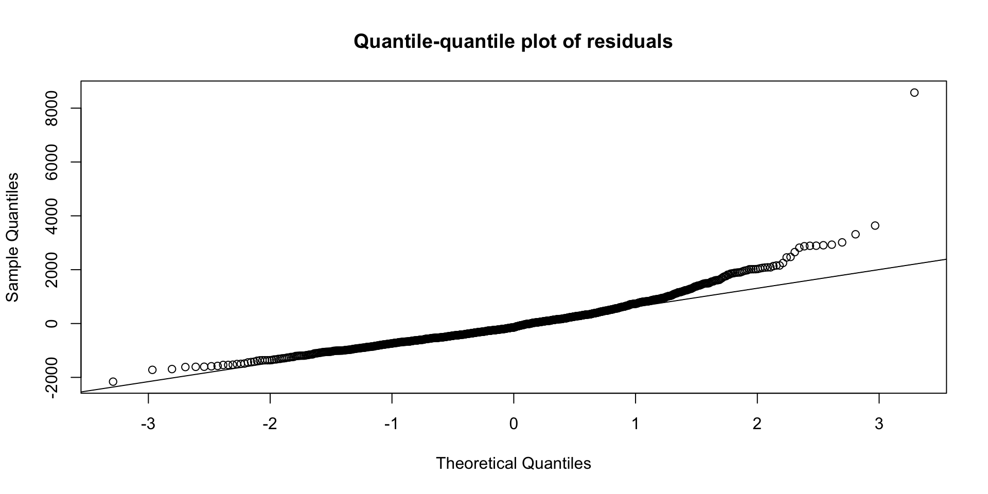
Code

qqnorm(residuals(lm1), main= "Quantile-quantile plot of residuals")
qqline(residuals(lm1))

What can we say about this graph?

Model fine-tuning

1. Independence: assumed by design;
2. Homoscedasticity: log transformation of energy
3. Normality: log transformation of energy
4. Linearity: restricted cubic spline transformation

Of note, log transformation not shown here for simplicity.

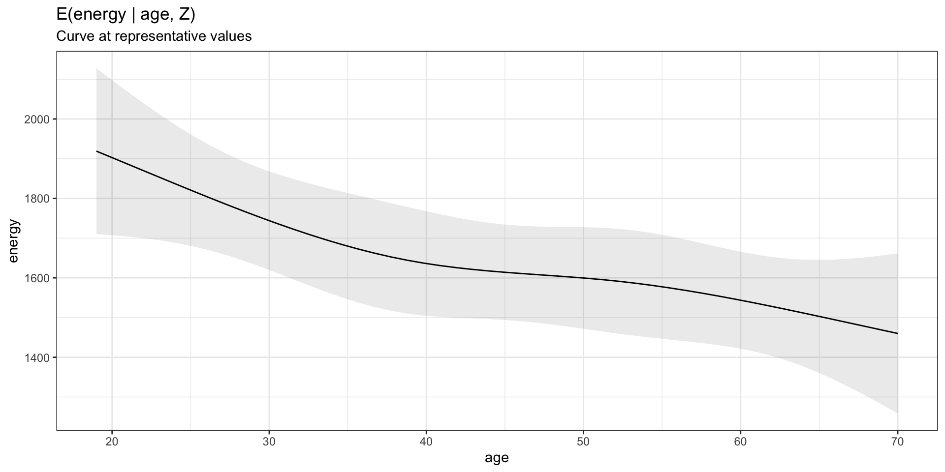
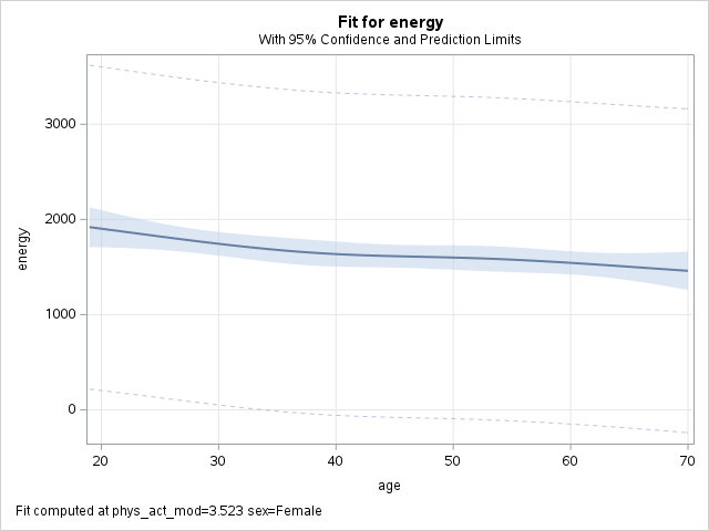
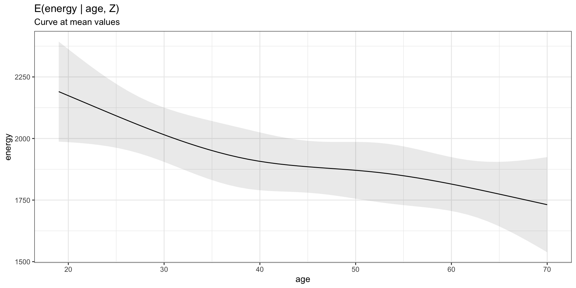
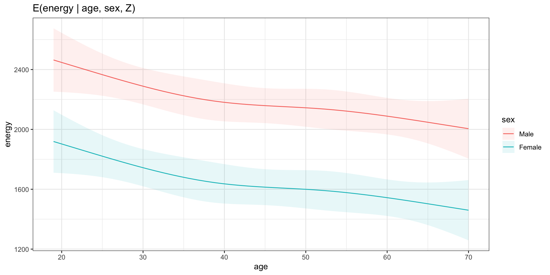
Revised model

Specify Restricted Cubic Spline (RCS) transformation with the rms package.

rms::rcs(variable,knots)

Code

# revised model
lm2 <- 
  glm(energy ~ rms::rcs(age,4) + sex + rms::rcs(phys_act_mod,3),
    family  = gaussian(link="identity") ,
    data    = final)

Exploring parameters: example

Code

gtsummary::tbl_regression(lm2)

Characteristic	Beta	95% CI1	p-value
Age, years
rms::rcs(age, 4)age	-16	-34, 1.0	0.065
rms::rcs(age, 4)age'	21	-26, 69	0.4
rms::rcs(age, 4)age''	-65	-234, 104	0.5
sex
Male	—	—
Female	-545	-653, -436	<0.001
Moderate or vigorous physical activity, hours/week
rms::rcs(phys_act_mod, 3)phys_act_mod	-13	-61, 36	0.6
rms::rcs(phys_act_mod, 3)phys_act_mod'	90	-34, 213	0.2
1 CI = Confidence Interval

… How can we interpret this revised model?

Categorical covariate/group mean (1)

Marginal Means/Least-square means: “Predictions of a model, averaged across a ‘reference grid’ of categorical predictors.”

Code

emmeans::lsmeans(lm2, "sex") 

 sex    lsmean   SE  df lower.CL upper.CL
 Male     2157 59.7 991     2040     2274
 Female   1612 61.2 991     1492     1733

Confidence level used: 0.95 

Categorical covariate/group mean (2)

More flexible analysis with marginaleffects

Code

marginaleffects::marginal_means(model = lm2, variables = "sex")

 Term  Value Mean Pr(>|z|) 2.5 % 97.5 %
  sex Male   2157   <0.001  2040   2274
  sex Female 1612   <0.001  1493   1732

Results averaged over levels of: sex 
Columns: rowid, term, value, sex, estimate, p.value, conf.low, conf.high, age, energy, phys_act_mod, wts 

Categorical covariate/group mean (SAS)

Least-Square Means: LS-means are predicted population margins—that is, they estimate the marginal means over a balanced population.

SAS equivalent: LSMEANS sex ;

Categorical covariate/group mean difference

Code

marginaleffects::marginal_means(model = lm2, variables = "sex",
                                hypothesis = "pairwise")

          Term Mean Pr(>|z|) 2.5 % 97.5 %
 Male - Female  545   <0.001   436    653

Results averaged over levels of: sex 
Columns: term, estimate, p.value, conf.low, conf.high 

SAS equivalent: LSMEANS sex / diff=all cl ;

Model visualization at representative values

Plot specific parameters with marginaleffects::plot_predictions

Code

  marginaleffects::plot_predictions(model = lm2,
                                    condition =c("age"),
                                    draw=TRUE)+
  ggplot2::labs(title="E(energy | age, Z)",
                subtitle = "Curve at representative values") +
  ggplot2::theme_bw() 

Model visualization at representative values (SAS)

SAS equivalent: proc plm ...;

Code

    proc plm restore=lm2  ;
        effectplot fit(x= age ) / clm at(sex="Female");
    run;

Model visualization at mean values

Alternative to representative values: use mean of all covariates, including categorical ones (coded as dummy covariates).

Code

# generate dummy-coded variable for sex
final$female <- ifelse(final$sex=="Female",1,0)

# revised model
lm2b <-
  glm(energy ~ rms::rcs(age,4) + female + rms::rcs(phys_act_mod,3),
    family  = gaussian(link="identity") ,
    data    = final)

• Age: mean(final$age)= 45.53
• Sex: mean(final$female) = 0.5
• Physical act.: mean(final$phys_act_mod) = 3.52

Model visualization at mean values

Code

  marginaleffects::plot_predictions(model = lm2b,
                                    condition =c("age"),
                                    draw=TRUE) +
  ggplot2::labs(title="E(energy | age, Z)",
                subtitle = "Curve at mean values") +
  ggplot2::theme_bw() 

Model visualization for more than 1 covariate

Code

  marginaleffects::plot_predictions(model = lm2,
                                    condition =c("age","sex"),
                                    draw=TRUE) + 
  ggplot2::labs(title="E(energy | age, sex, Z)") +
  ggplot2::theme_bw()

Custom hypothesis at user-defined values

Use marginaleffects::avg_comparisons

E(energy|age=60, Z) - E(energy|age=30, Z)

Code

# <avg_comparisons> to calculate estimated Y given X and average Z
marginaleffects::avg_comparisons(lm2,
                                 variables = list(age = c(30,60))
                                 ) 

 Term Contrast Estimate Std. Error     z Pr(>|z|) 2.5 % 97.5 %
  age  60 - 30     -200       68.9 -2.91  0.00365  -335  -65.2

Columns: term, contrast, estimate, std.error, statistic, p.value, conf.low, conf.high 

Custom hypothesis for common change

E(energy|age=75^th, Z) - E(energy|age=25^th, Z)

Code

# <avg_comparisons> to calculate estimated Y given X and average Z
marginaleffects::avg_comparisons(lm2,
                                 variables = list(age = "iqr"))

 Term Contrast Estimate Std. Error     z Pr(>|z|) 2.5 % 97.5 %
  age  Q3 - Q1     -126       78.2 -1.61    0.107  -279   27.3

Columns: term, contrast, estimate, std.error, statistic, p.value, conf.low, conf.high 

More examples available online

Example 2: more complex model

For causal inference purpose, we wish to estimate the risk of hypertension across the range of sodium intakes.

Model (estimator): \(\text{logit}(\pi)=\beta_0+\beta_\text{Na}\text{Na}+\gamma Z\)

Hypothesized relationship

Assume temporality and that this causal directed acyclic graph (DAG) is correct:

• \(\text{Na}\) sodium intake (mg)
• \(\text{HBP}\) High blood pressure
• \(U\) (unobserved) propensity towards health-seeking behaviors
• \(Z_1\) age, sex, university education level
• \(Z_2\) smoking, moderate/intense physical activity

Prepare data

Combine variables to avoid over-fitting, i.e., limiting sample size = 142 events (Harrell 2015).

Code

# recode categorical covariates
final <- 
  final |>
  dplyr::mutate(
    # education: university vs. else
    edu_4 = ifelse(education==4,1,0),
    # smoking: daily or occasional smoker vs. else
    smk_1 = ifelse(smoking %in% c(1,2),1,0)
  )

# confirm recoding
with(final,table(edu_4,education))

     education
edu_4   1   2   3   4
    0  84 258 348   0
    1   0   0   0 300

Code

with(final,table(smk_1,smoking))

     smoking
smk_1   0   1   2
    0 802   0   0
    1   0  50 148

Logistic regression model

Code

logm1 <-
  glm(self_reported_bp ~ rms::rcs(sodium,3) + rms::rcs(age,3) + female + 
          edu_4 + smk_1 + rms::rcs(phys_act_mod,3),
      binomial(link = "logit"),
      data = final )

logm1

Call:  glm(formula = self_reported_bp ~ rms::rcs(sodium, 3) + rms::rcs(age, 
    3) + female + edu_4 + smk_1 + rms::rcs(phys_act_mod, 3), 
    family = binomial(link = "logit"), data = final)

Coefficients:
                           (Intercept)               rms::rcs(sodium, 3)sodium  
                            -9.7611025                               0.0004064  
            rms::rcs(sodium, 3)sodium'                     rms::rcs(age, 3)age  
                            -0.0006629                               0.1621546  
                  rms::rcs(age, 3)age'                                  female  
                            -0.0635853                              -0.3261307  
                                 edu_4                                   smk_1  
                            -0.3632489                              -0.3183342  
 rms::rcs(phys_act_mod, 3)phys_act_mod  rms::rcs(phys_act_mod, 3)phys_act_mod'  
                             0.0329085                              -0.0477153  

Degrees of Freedom: 986 Total (i.e. Null);  977 Residual
  (13 observations deleted due to missingness)
Null Deviance:      798.7 
Residual Deviance: 642.3    AIC: 662.3

:::

Model visualization at mean values

Code

marginaleffects::plot_predictions(model = logm1, condition =c("sodium"),
                                  draw=TRUE) +
# Limit axis to remove extreme values 
ggplot2::coord_cartesian(xlim=c(quantile(final$sodium,0.01),
                                quantile(final$sodium,0.99))) +
# Add labels
ggplot2::labs(title    = "Pr(High blood pressure | sodium, Z)",
              subtitle = "Curve at mean values",
              x = "Sodium intake, mg",
              y = "Probability of high blood pressure") +
ggplot2::theme_bw() 

Conclusion

• Don’t stop at standard output regression model
• Marginal effects facilitate communication
• Create graph and/or test custom hypothesis
  • R: marginaleffects + ggplot2
  • SAS: option store + proc plm + proc sgplot
  • SAS: option estimate + ods output <...>;

References

Arel-Bundock, Vincent. 2023. Marginaleffects: Predictions, Comparisons, Slopes, Marginal Means, and Hypothesis Tests. https://vincentarelbundock.github.io/marginaleffects/.

Harrell, F. E. 2015. Regression Modeling Strategies: With Applications to Linear Models, Logistic Regression, and Survival Analysis. Book. Springer International Publishing. https://books.google.ca/books?id=kfHrF-bVcvQC.

Norton, E. C., B. E. Dowd, and M. L. Maciejewski. 2019. “Marginal Effects-Quantifying the Effect of Changes in Risk Factors in Logistic Regression Models.” Journal Article. JAMA 321 (13): 1304–5. https://doi.org/10.1001/jama.2019.1954.