
‘Statistical method you should know’: the bootstrap
Published:
In this article, I describe a statistical method that I use very often: the bootstrap. Yet, I believe the method is rarely thought outside epidemiology or biostatistics graduate studies curriculum. This is unfortunate because the bootstrap is (relatively) simple and extremely useful.
Disclaimer: I have a PhD in nutrition, thus my knowledge of statistical methods is that of a naive enthusiast at best. I aim to provide a practical introduction based on my understanding. Please correct me where needed.

Efron and Tibshirani (1994) states that the “bootstrap is a computer-based method for assigning measures of accuracy to statistical estimates”. Informally, I describe the bootstrap as a statistical method to estimate variance of any given statistic using resampling. Let’s dissect that statement.
First, “to estimate variance” refers to calculating standard errors and confidence intervals. Typically, we calculate standard errors assuming an underlying probability distribution, e.g., normal/Gaussian. Assuming some distribution, we can then use formula to derive standard errors (theoretical standard errors). However, the bootstrap method does not need to rely on these assumed distributions.;
Second, “any given statistic” is what makes bootstrap methods extremely useful! We can use it to estimate variance of statistics for which we do not have formula to derive variance. For example, it is less common to have built-in variance estimates for a median, a difference between two medians or other quantiles. The bootstrap is also relevant to properly obtain variance of a multistep analysis; again, for which we would not have formula to derive theoretical standard errors and confidence intervals. Some examples of multistep analysis are prediction analysis (variable selection, prediction, …), causal inference (propensity score estimation, outcome model) or measurement error correction (transformation, error model, distribution estimation or outcome model).
Third, “using resampling” is the core of bootstrap methods. One way to use the boostrap is to generate multiple new datasets from the original dataset and based on a sampling scheme consistent with that of the original dataset. However, the resampling process is performed with replacement, i.e., the same unit can be selected more than once. In other words, the idea is to repeat the sampling process that led to the original sample to create many new samples of the same size (same n) as the original. These new samples then allow us to estimate standard errors or confidence intervals.
I won’t go into more theoretical details before I embarrass myself. Relevant references to learn more include the 1-page BMJ Statistic Notes (Bland and Altman, 2015), the An Introduction to the Bootstrap book (Efron and Tibshirani, 1994), or the original paper of the method by Efron (1979).
Schematic overview
The figure below illustrates the steps needed for a bootstrap analysis.
flowchart TD
    A([Target population]) --Sampling--> B(Original
study sample
of size n)
    B --Resampling
with replacement
B times--> C("B 'bootstrap samples'
of size n")
    C --> B
    C --Repeat in each
bootstrap sample--> D[Analysis]
    D --> C
    D --> E[B times the statistic
of interest for
variance estimation via...]
    E --> E1[Percentile
method]
    E --> E2[Normal
approximation]
    E --> E3[...]
Data overview
The simple example below should help clarify my vague description of the method. For simplicity, I use the built-in R data set mtcars (“fuel consumption and 10 aspects of automobile design and performance for 32 automobiles (1973–74 models”) and R code. Say that this data is a simple random sample of cars available at the time. We might be interested in drawing inference about the horsepower of these cars.
# ********************************************** #
#                 Data overview                  #
# ********************************************** #

# 5 observations
head(mtcars)
                   mpg cyl disp  hp drat    wt  qsec vs am gear carb
Mazda RX4         21.0   6  160 110 3.90 2.620 16.46  0  1    4    4
Mazda RX4 Wag     21.0   6  160 110 3.90 2.875 17.02  0  1    4    4
Datsun 710        22.8   4  108  93 3.85 2.320 18.61  1  1    4    1
Hornet 4 Drive    21.4   6  258 110 3.08 3.215 19.44  1  0    3    1
Hornet Sportabout 18.7   8  360 175 3.15 3.440 17.02  0  0    3    2
Valiant           18.1   6  225 105 2.76 3.460 20.22  1  0    3    1
# number of rows (i.e., cars) and columns (i.e., variables)
dim(mtcars)
[1] 32 11
# ********************************************** #
#              Horsepower overview               #
# ********************************************** #

# Mean
mean(mtcars$hp)
[1] 146.6875
# Range and distribution
range(mtcars$hp)
[1] 52 335
hist(mtcars$hp, main="Horsepower distribution of cars in mtcars")
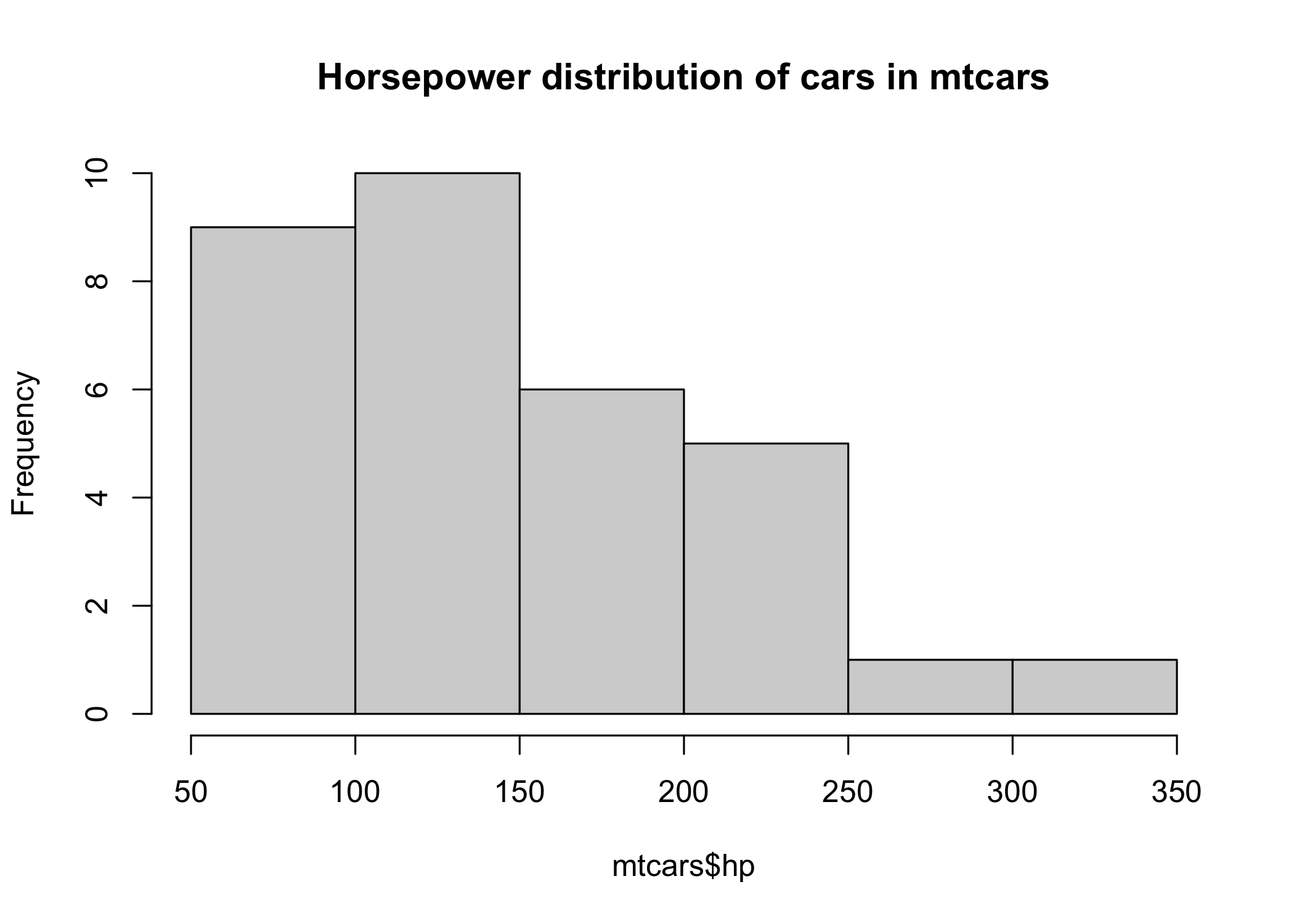
We can see that 1) the distribution is right-skewed; 2) should we assume a Gaussian distribution to derive a confidence interval, it would probably not fit the data very well.
Of note, for simplicity, I use the mean to demonstrate the bootstrap method. However, remember that it could be used for any statistics, even those for which software typically don’t have built-in theoretical confidence intervals.
Resampling example
Resampling by hand
The core of the bootstrap method is that, since we obtained a random sample of cars in the first place (from a hypothetical population of cars), we can randomly sample with replacement cars directly from the sample we have. The new samples created would be no different than the one we originally obtained from the population.
In each resample, some cars will appear more than once - they will appear as they were “repeated observations” - and other cars may never be selected. Weirdly, this is fine as long as the resampling (here, simple random sampling) is consistent with the original sampling and done with replacement. The new bootstrap samples should also have the same number of observations than the original sample.
library(dplyr)
library(ggplot2)

# ********************************************** #
#               Manual resampling                #
# ********************************************** #

# (1) Randomly select rows with replacement from the original sample
## Set seed results are reproducible
set.seed(1)
## resampling
mtcars_rows1 <-
  sample( x = 1:nrow(mtcars),   # row numbers
          size = nrow(mtcars),  # number of observations in original data
          replace = TRUE # sample with replacement
          ) |>
  as_tibble() |>
  # add an identifier for bootstrap sample
  mutate(
    replicate=1
  )

# (2) Randomly select rows with replacement from the original sample
## Set seed results are reproducible
set.seed(2)
## resampling
mtcars_rows2 <-
  sample( x = 1:nrow(mtcars),   # row numbers
          size = nrow(mtcars),  # number of observations in original data
          replace = TRUE # sample with replacement
          ) |>
  as_tibble() |>
  # add an identifier for bootstrap sample
  mutate(
    replicate=2
  )

# (0) Generate data illustrating the original sample
mtcars_original <-
  # each cars appear once in the original sample
  data.frame(value = seq(1,32,1),
             # bootstrap identifier = 0  for the original sample
             replicate = 0)

# Combine 1 bootstrap sample with original sample
original_and_bootstrap <-
  rbind(mtcars_original,mtcars_rows1,mtcars_rows2)

  ## apply formatting for clarity
  original_and_bootstrap$replicate_f <-
    factor(original_and_bootstrap$replicate,
           levels = c(0,1,2),
           labels = c("Original sample, n=32",
                      "First bootstrap sample, n=32",
                      "Second bootstrap sample, n=32"))

# ********************************************** #
#          Create graph to show process          #
# ********************************************** #

# Show graph to see which rows were selected vs. original
  ggplot(data=original_and_bootstrap,aes(value)) +
    geom_dotplot(binwidth = 1,color="black",fill="gray") +
    scale_x_continuous(limits=c(1,32),breaks=seq(1,32,1)) +
    scale_y_continuous(NULL, breaks = NULL) +
    ## Show samples on different rows
    facet_wrap(~replicate_f,ncol=1) +
    labs(title = "Original vs. bootstrap samples (with replacement) of 32 cars in mtcars",
         subtitle = "Dots indicate the number of times a car was selected",
          x="Car identifier, 1 to 32",
          caption="Stacked dots: >1 selection\nNo dots (empty space): not selected") +
    ## theme and formatting
    theme_bw(base_size = 12) +
    theme(
      panel.grid.minor = element_blank(),
      strip.background = element_rect(fill="black"),
      strip.text = element_text(color="white", face="bold")
    )
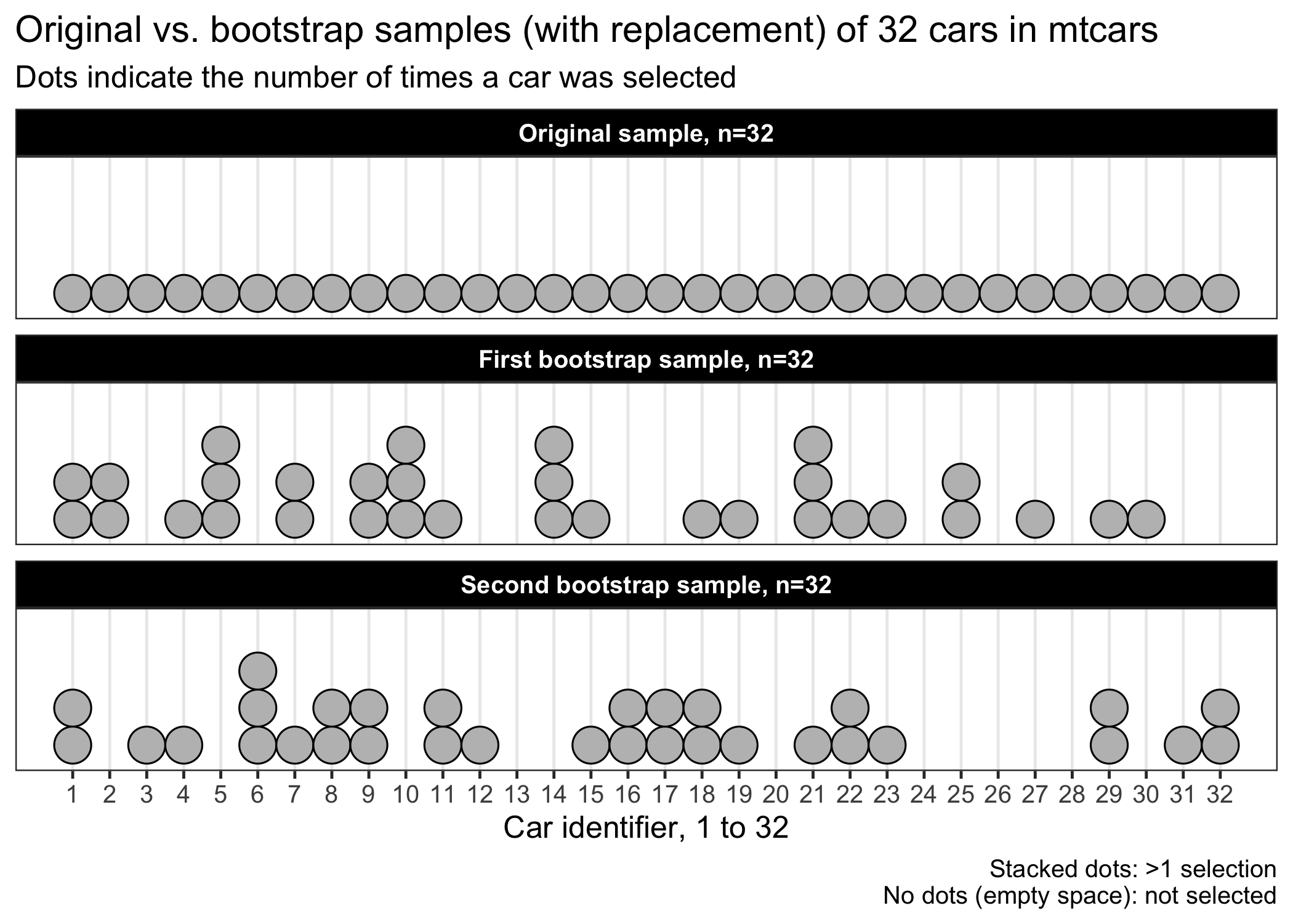
When we compare the two bootstrap samples with the original sample, we see that some cars were picked more than once (stacked dots in the figure), while others were not (empty spaces). The mean horsepower in the first bootstrap sample is 143, while the mean horsepower is 147 HP in the original sample. Informally, we can interpret the bootstrap samples as just another sample that we could have obtained, had we sampled the same number of cars again from the hypothetical larger population of cars.
Of note, there is only one sample in the mtcars example. However, sometimes there are two samples as in the case of a randomized experiment with two interventions. Accordingly, we would have to perform simple random sampling within each intervention arms to create bootstrap samples based on such design (Efron and Tibshirani, 1994). All in all, the bootstrap resampling must be consistent with the original sampling, but performed with replacement.
How many resamples do we need?
The downside of the bootstrap is that we need a large number of resamples on which we repeat the analysis. Generating a large number of bootstrap samples, say a thousand, and calculating the mean horsepower in each of these new samples is very fast in this example. Indeed, the sample size is small (n=32) and the analysis is very simple (i.e., calculating the mean).
However, for a computationally intensive analysis or when dealing with very large data sets, sometimes only 100 or 200 bootstrap samples are used. For most purpose, it seems that 200 bootstrap samples could be enough (Efron and Tibshirani, 1994), but more doesn’t hurt if it is not a problem.
Example 1: the mean
Packages are available in R to do an efficient bootstrap analysis. Here, I show how to do a simple bootstrap analysis using the boot package
# ********************************************** #
#          Bootstrap analysis with BOOT          #
# ********************************************** #

# load needed library
library(boot)
library(tibble)

# set seed for reproducibility
set.seed(123)

# Decide on a number of bootstrap resamples
number_of_resamples <- 1000

# Function which gives the sample mean
my_analysis <- function(data,ind) { mean(data[ind,"hp"]) }

    # note: <hp> is hardcoded so the function is not flexible for additional analyses

# Perform bootstrap resampling and calculation using the BOOT function

tictoc::tic()

    #note: <tictoc> package is useful to assess analysis time

my_analysis_bootstrap <-
  boot::boot(data = mtcars, # data with variable of interest
       statistic = my_analysis, # the analysis to perform
       R = number_of_resamples , # number of bootstrap replicates (new samples)
       stype = "i", # indicate that the second argument in <my_analysis> is for row indices
       parallel = "multicore", # ask parallel analysis (faster with complex analysis)
       ncpus = parallel::detectCores()-1 # detect cores available
       )

    # note: parallel computing is overkill here, but could be relevant with more complex analysis

tictoc::toc()
0.059 sec elapsed
# ********************************************** #
# Check analysis output #
# ********************************************** #
# Look at the output
my_analysis_bootstrap$t |>
tibble::as_tibble_col() |>
ggplot(aes(value)) +
geom_histogram(binwidth = 5, aes(y=..density..), colour="black",fill="#e67424") +
geom_vline(xintercept=my_analysis_bootstrap$t0,linetype="longdash") +
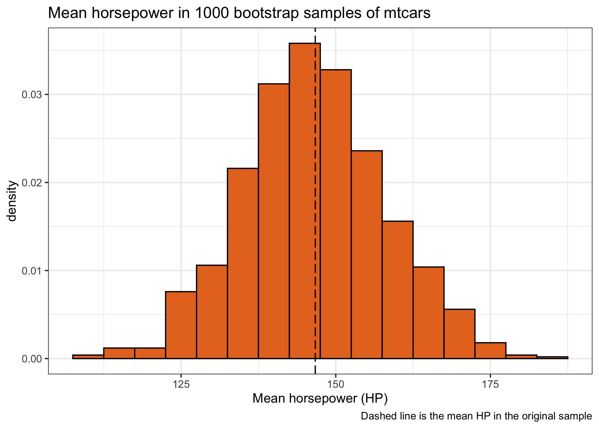
labs(title = paste0("Mean horsepower in ",number_of_resamples," bootstrap samples of mtcars"),
x="Mean horsepower (HP)",
caption = "Dashed line is the mean HP in the original sample") +
theme_bw()
my_analysis_bootstrap$t |>
  tibble::as_tibble_col() |>
  ggplot(aes(sample=value)) +
  stat_qq() + stat_qq_line() +
  labs(title = paste0("Normal quantile-quantile of mean horsepower in ",
                      number_of_resamples," bootstrap samples of mtcars"),
       x="Normal quantile",
       y="Mean horsepower (HP)") +
  theme_bw()
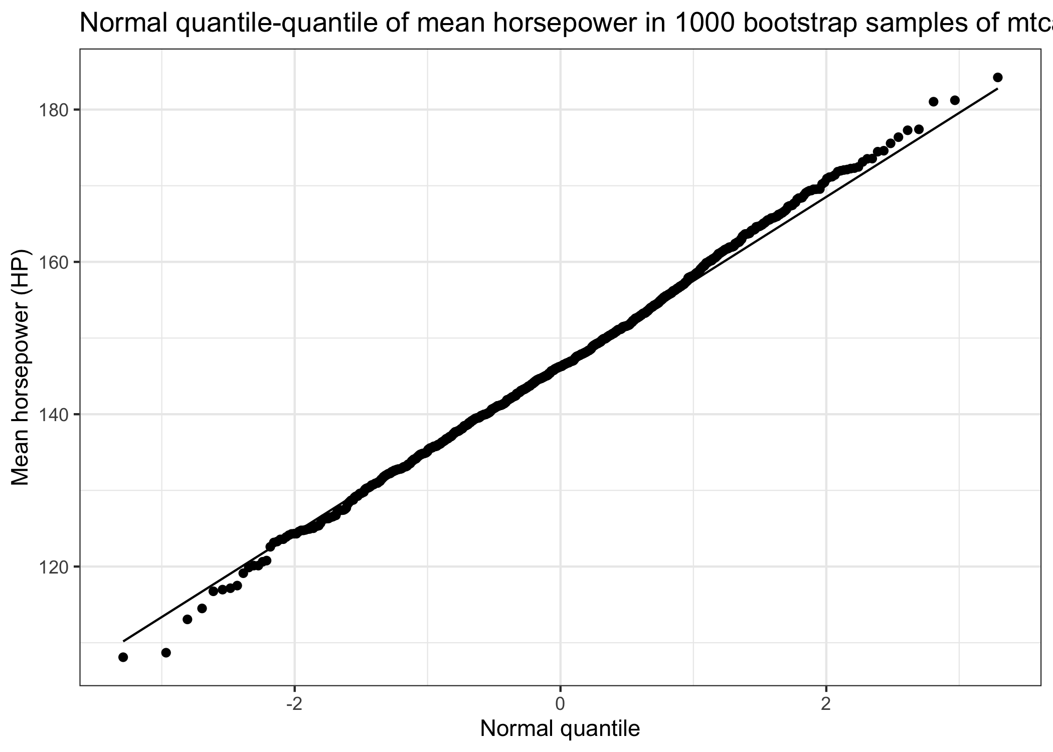
An interesting observation is that the distribution of the mean horsepower of many bootstrap samples (also called the sampling distribution) has a very normal/Gaussian distribution, although the distribution of horsepower in the original sample was skewed. We can use this nice bootstrap distribution to estimate confidence intervals. There are different ways to obtain these variance estimates, but I show on two common methods: the percentile method and the normal approximation.
Output confidence intervals
# ********************************************** #
#              Confidence intervals              #
# ********************************************** #

# Calculate confidence intervals using PERCENTILE (the 2.5th and 97.5th quantile)
boot_variance_perc <-
  boot.ci(my_analysis_bootstrap,
        type="perc")

  ## export confidence intervals
  bootvar_perc <-
    boot_variance_perc$percent |>
    tibble::as_tibble()

boot_variance_perc
BOOTSTRAP CONFIDENCE INTERVAL CALCULATIONS
Based on 1000 bootstrap replicates

CALL :
boot.ci(boot.out = my_analysis_bootstrap, type = "perc")

Intervals :
Level     Percentile
95%   (124.6, 170.2 )
Calculations and Intervals on Original Scale
# Calculate confidence intervals using NORMAL APPROXIMATION (1.96*Standard Deviation)
boot_variance_norm <-
  boot.ci(my_analysis_bootstrap,
        type="norm")

  ## export confidence intervals
  bootvar_norm <-
    boot_variance_norm$normal |>
    tibble::as_tibble()

boot_variance_norm
BOOTSTRAP CONFIDENCE INTERVAL CALCULATIONS
Based on 1000 bootstrap replicates

CALL :
boot.ci(boot.out = my_analysis_bootstrap, type = "norm")

Intervals :
Level      Normal
95%   (124.1, 169.6 )
Calculations and Intervals on Original Scale
# For comparison purpose, calculate theoretical 95%CI
 theoretical_se <- sd(mtcars$hp)/sqrt(nrow(mtcars))
 mean <- mean(mtcars$hp)
 theoretical_lcl <- round(mean - theoretical_se*1.96)
 theoretical_ucl <- round(mean + theoretical_se*1.96)
The percentile method (95%CI: 125 to 170) and the normal approximation (95%CI: 124 to 170) produced similar confidence intervals. The normal approximation works well in this example, because the bootstrap distribution of mean is close to a normal distribution. For simple statistics like the mean, this is often the case.
Finally, the 95% confidence interval calculated using theoretical standard errors (\(StdErr = StdDev/\sqrt n\)) and normal approximation (\(CL=1.96\cdot StdErr\)) is 123, 170. The theoretical confidence interval is almost identical compared to the bootstrap confidence interval. What!? Why did with bother calculating bootstrap confidence intervals then? Well, first, it is a good thing that the theoretical formula for mean works as intended and, second, remember there is no formula for many other complex statistics! For example, the code below demonstrates how the bootstrap could help obtain median difference with confidence interval.
Example 2: median difference and confidence intervals
# Hypothetical question:
# What is the median difference in horsepower for cars with 4 cylinders vs. more than 4 cylinders?

# ********************************************** #
#    Prepare data and `boot` for median diff.    #
# ********************************************** #

# Copy mtcars data
mtcars_flag <- mtcars

# Flag cars according to the number of cylinder
mtcars_flag$more_than_4cyl <-
  ifelse(mtcars_flag$cyl > 4,1,0)
  # reads as: if value of "cyl" is greater than 4, assign 1 to "more_than_4cyl", otherwise, assign 0

# Create function which gives median (by cylinder group) and difference
my_analysis2 <- function(data,ind) {
  data[ind,] |>
  # group by <more_than_4cyl> (i.e., 4 cyl. OR more than 4 cyl.)
  dplyr::group_by(more_than_4cyl) |>
  # calculate median for each group
  dplyr::summarise(medianHP = median(hp)) |>
  # transpose to "wide" foramt to calculate difference
  tidyr::pivot_wider(names_from=more_than_4cyl,
                     values_from=medianHP,
                     names_prefix="cyl") |>
  # actual difference
  dplyr::mutate(
    median_diff = cyl1 - cyl0
  ) |>
  # keep only the median_diff value
  dplyr::pull(median_diff)
  }

# Perform bootstrap resampling and calculation using the BOOT function
tictoc::tic()

my_analysis2_bootstrap <-
  boot::boot(data = mtcars_flag, # data with variable of interest
       statistic = my_analysis2, # the analysis to perform
       R = 1000 , # number of bootstrap replicates (new samples)
       stype = "i", # indicate that the second argument in <my_analysis> is for row indices
       parallel = "multicore", # ask parallel analysis (faster with complex analysis)
       ncpus = parallel::detectCores()-1 # detect cores available
       )

    # note: parallel computing is 3-4x faster than not in this example
tictoc::toc()
5.591 sec elapsed
# ********************************************** #
#              Confidence intervals              #
# ********************************************** #

# Estimate of median difference (original sample)
  my_analysis2_bootstrap$t0
[1] 84
# Calculate confidence intervals
  ## Normal approximation
  boot.ci(my_analysis2_bootstrap,
          type="norm")
BOOTSTRAP CONFIDENCE INTERVAL CALCULATIONS
Based on 1000 bootstrap replicates

CALL :
boot.ci(boot.out = my_analysis2_bootstrap, type = "norm")

Intervals :
Level      Normal
95%   ( 38.26, 114.99 )
Calculations and Intervals on Original Scale
  ## Percentile
  boot.ci(my_analysis2_bootstrap,
          type="perc")
BOOTSTRAP CONFIDENCE INTERVAL CALCULATIONS
Based on 1000 bootstrap replicates

CALL :
boot.ci(boot.out = my_analysis2_bootstrap, type = "perc")

Intervals :
Level     Percentile
95%   ( 47.15, 126.50 )
Calculations and Intervals on Original Scale
Of note, the bootstrap distribution of median difference is not very consistent with a normal distribution (not shown). Hence there are differences between confidence intervals for the “normal” and “percentile” methods. The percentile method may be more appropriate in this case.
Based on the analysis above, we conclude that cars with more than 4 cylinders had a +84 higher (median) HP than cars with 4 cylinders. The 95%CI shows that the data are compatible with a median difference of 47 to 126.
References
Bland J. M. and Altman D. G. Statistics Notes: Bootstrap resampling methods BMJ 2015; 350: h2622 doi: 10.1136/bmj.h2622.
Efron, B. (1979) Bootstrap Methods: Another Look at the Jackknife. The Annals of Statistics, 7(1), 1-26.
Efron, B. and Tibshirani, R. J. (1994) An Introduction to the Bootstrap, 1st edition. Chapman and Hall/CRC. doi: 10.1201/9780429246593