
Analyzing the Canadian Community Health Survey (CCHS) 2015 data with R: linear regression example
Published:
A key component of survey analysis, including the CCHS 2015 - Nutrition (Health Canada 2017) is accounting for the survey design. Indeed, the design must be properly specified to obtain proper standard errors and variance estimates. Plus, using the sampling weights generates estimates representative of the target population. SAS is often the go-to statistical package for complex sampling survey analysis. In my experience, introductory workshops on survey analysis teach how to use SAS’ PROC SURVEYMEANS, PROC SURVEYREG, etc. However, examples in R are often not provided. Recently, I have been using R a lot more, but I struggled to find good example for the CCHS 2015 - Nutrition.
The goal of this post is to save you some time and provide you with code on how to specify the Canadian Community Health Survey (CCHS) 2015 design to do a simple analysis. In R, we can analyze complex sampling survey data with the survey package (Lumley 2020).
Note that data for the CCHS 2015 - Nutrition (Public Use Micro Datafile or PUMF) are publicly available.
Simple analysis
For demonstration purpose, I focus on a simple analysis where we would be interested in the relationship between self-reported energy intakes on a given day (kcal), age (years) and biological sex (male or female). In other words, the objective is to describe the expected value of energy intake (\(Y_i\)) according to age (\(X_i\)) and covariate sex (\(Z_i\)) using linear regression in the form of:
\[Y_i=\beta_0 + \beta_{X_i} X_i + \beta_{Z_i} Z_i +\epsilon_i\]Key elements of survey analysis
There are 3 main components for a survey analysis based on the CCHS data:
Data: the variables energy intakes, age and sex for this example;
Sampling weights: the
WTS_Pvariable for the present PUMF data (orWTS_Mfor the masterfile available in Research data center). The sampling weights allow estimates to be representative of the target Canadian population at the time of the survey;Bootstrap replicate weights: 500 variables
BSW1-500which are varying weights for all individuals according to bootstrap samples. These variables are mandatory to obtain proper variance estimate (e.g., Standard Errors or Confidence Intervals).
Below, I show how to load the data in R. The HS datafile includes sociodemographic characteristics and summary dietary intake data (e.g., total energy consumed on a given day). Note that the sampling weight variable WTS_P is already included in HS. For variance estimation, the CCHS 2015 used the bootstrap method and bootstrap replicate weights. Other surveys like NHANES sometimes provide the sampling frame (variables for strata, cluster). Such variables are not available in CCHS 2015 for confidentiality purpose I believe. Regardless, I show how to import bootstrap replicate weight (the b5 data).
Loading packages and data
# ********************************************** #
#             Load required packages             #
# ********************************************** #

library(dplyr)
library(data.table)
library(parallel)
library(survey)
library(ggplot2)
library(gt)
library(haven)
library(parameters)
library(marginaleffects)

# ********************************************** #
#         Load and prepare CCHS data: HS         #
# ********************************************** #

  # Note: a hardcoded path (<external_drive>) is used since files are on an external drive.
  # Usually we would want analysis to be self-contained, but survey files are a bit large.
  # Also, the data are set-up exactly as they are once obtained from Statistics Canada

# HS data file (includes energy intakes, age, sex, sampling weights)
cchs_data <-
  haven::read_sas(data_file = file.path(external_drive,"CCHS_Nutrition_2015_PUMF","Data_Donnee","hs.sas7bdat"),
                  col_select = c(ADM_RNO,WTS_P,DHH_AGE,DHH_SEX,FSDDEKC)) |>
  ## rename variables for simplicity
  dplyr::rename(AGE = DHH_AGE,
                SEX = DHH_SEX,
                ENERGY = FSDDEKC ) |>
  ## keep respondents aged 19-70y only, non-null energy
  dplyr::filter(AGE>18, AGE<71, ENERGY>0) |>
  ## create an indicator variable with value of 1 for sex=males, 0 otherwise
  dplyr::mutate(
    MALE = ifelse(SEX==1,1,0)
  )

# ********************************************** #
#         Load and prepare CCHS data: B5         #
# ********************************************** #

# Bootstrap replicate weights (for variance estimation)
 bsw <-
   data.table::fread(file.path(external_drive,"CCHS_Nutrition_2015_PUMF","Bootstrap",
                               "Data_Donnee","b5.txt"),
                     stringsAsFactors = F, data.table= F, header=F,
                     nThread = parallel::detectCores()-1, # note: a bit overkill, but why not
                     col.names = c("ADM_RNO","WTS_P",paste0("BSW",seq(1,500)))) |>
   # keep only respondents identified above
   dplyr::right_join(cchs_data[,"ADM_RNO"]) |>
   # remove sampling weights so that only 1 copy exists in <cchs_data>
   dplyr::select(-WTS_P)
Understanding survey data
With survey data, each respondent has an analytical weight (or sampling weight) attributed according to individual characteristics. A single survey respondent represents as many individuals in the target population as the value of the analytical weight in a given analysis. For example, for the first respondent in our data, the value of WTS_P is 859 which indicates that this respondent provides information meant to reflect approximately 859 individuals in the target population. The bootstrap replicate weights are also analytical weight for each respondent, but based on a resample data.
# ********************************************** #
#             Overview of HS and BSW             #
# ********************************************** #

 # cchs_data overview
 head(cchs_data)
# A tibble: 6 × 6
  ADM_RNO   AGE   SEX WTS_P ENERGY  MALE
    <dbl> <dbl> <dbl> <dbl>  <dbl> <dbl>
1       1    27     2   859  3122.     0
2       2    48     1   901  2880.     1
3       4    39     2   539  1658.     0
4       5    28     1   703  3712.     1
5       6    52     2    42  1446.     0
6       7    40     2  1949  2686.     0
 # bootstrap weight overview
 head(bsw[,1:6])
  ADM_RNO BSW1 BSW2 BSW3 BSW4 BSW5
1       1   31   33 2234   27 1804
2       2  539   62   64   60  807
3       4   50   33   42 1941 2074
4       5   50 1812   64   60 2010
5       6  312  188  144  225  172
6       7 3903 4155   30 6221   29
Specifying the survey design
This step is crucial to obtain accurate estimates and variance. We use the function svrepdesign to specify a survey design based on replicate weights. Of note, in a survey design with replicate weights, the default option to calculate standard errors is to take “squared deviations between the replicates and their mean, not deviations between the replicates and the point estimate”, i.e., mse=FALSE in svyrepdesign (Lumley 2010). However, SAS calculates standard errors using the latter approach. For compatibility purpose with SAS’ estimates, I set mse=TRUE in this example.
# ********************************************** #
#             Specify survey design              #
# ********************************************** #

  cchs_design_bsw <-
    survey::svrepdesign(
      data =  cchs_data, # HS data with variables of interest + sampling weights
      type = "bootstrap", # Replicate weights are bootstrap weights in CCHS
      weights    = ~WTS_P, # Sampling weights
      repweights = bsw[,2:501], # Bootstrap replicate weights (i.e. BSW1, BSW2, ... BSW500)
      combined.weights=TRUE,  # in CCHS 2015, weights are combined
      mse = TRUE # 'compute variances based on sum of squares around the point estimate' = same as in SAS
      )

# ********************************************** #
#              Check Survey Object               #
# ********************************************** #

cchs_design_bsw
Call: svrepdesign.default(data = cchs_data, type = "bootstrap", weights = ~WTS_P,
    repweights = bsw[, 2:501], combined.weights = TRUE, mse = TRUE)
Survey bootstrap with 500 replicates and MSE variances.
Main analysis
Once the survey design is specified, we can go on with the analysis. I use survey::svyglm which is the survey analog of base R’s Generalized Linear Models function glm. The SAS equivalent is PROC SURVEYREG.
# ********************************************** #
#        Linear regression model example         #
# ********************************************** #

svy_lm <-
  survey::svyglm(ENERGY ~ AGE + MALE,
                 design = cchs_design_bsw,
                 multicore = TRUE, # slightly faster
                 family = gaussian(link="identity"))

# Show simple model summary
svy_lm |>
  summary()
Call:
survey::svyglm(formula = ENERGY ~ AGE + MALE, design = cchs_design_bsw,
    multicore = TRUE, family = gaussian(link = "identity"))

Survey design:
svrepdesign.default(data = cchs_data, type = "bootstrap", weights = ~WTS_P,
    repweights = bsw[, 2:501], combined.weights = TRUE, mse = TRUE)

Coefficients:
            Estimate Std. Error t value            Pr(>|t|)
(Intercept) 1905.112    137.360  13.869 <0.0000000000000002 ***
AGE           -6.181      2.871  -2.153              0.0318 *
MALE         585.350     43.925  13.326 <0.0000000000000002 ***
---
Signif. codes:  0 '***' 0.001 '**' 0.01 '*' 0.05 '.' 0.1 ' ' 1

(Dispersion parameter for gaussian family taken to be 662136.3)

Number of Fisher Scoring iterations: 2
# Output parameter estimates in a data
  svy_lm_parm <-
    parameters::model_parameters(svy_lm) |>
    tibble::as_tibble()
The linear model above indicates that 1-y increase in age is associated with a 6 kcal lower self-reported energy intake (95%CI: -12, -1). Being a male is also associated with a 585 kcal greater energy intake (95%CI: 499, 672). This observation is consistent with the fact that males tend to be taller, to have higher bodyweight and, thus, to report eating more foods. The model intercept (1905 kcal) corresponds to the expected reported energy intake when age=0 and male=0, i.e., a 19-y female in the present example. This seems quite low, but is not expected given the documented underreporting of energy intake in CCHS 2015 - Nutrition (Garriguet 2018).
For a scientific publication, we would probably want to clean the output a bit to obtain a table of model coefficients. Below is a draft code to output a formatted table.
# ********************************************** #
#       Linear regression model parameters       #
# ********************************************** #

# Output table
  svy_lm_parm |>
    dplyr::select(-c(CI,Statistic,df_error,p)) |>
    gt::gt() |>
      gt::cols_label(
        SE = "Standard Error",
        CI_low = "Lower",
        CI_high = "Upper"
      ) |>
      gt::tab_spanner(
        label = "95% Confidence intervals",
        columns = c(CI_low,CI_high),
      ) |>
      gt::fmt_number(col=c(Coefficient,SE,CI_low,CI_high),decimals=0) |>
      gt::tab_header(
        title = "Linear regression models of reported energy intake on age and sex in adults 19-70 y from the CCHS 2015 - Nutrition") |>
      gt::tab_source_note(
        source_note = "Adapted from Statistics Canada, Canadian Community Health Survey - Nutrition:
        Public Use Microdata File, 2015, October 2022.
        This does not constitute an endorsement by Statistics Canada of this product") |>
      gt::opt_align_table_header("left")
| Linear regression models of reported energy intake on age and sex in adults 19-70 y from the CCHS 2015 - Nutrition | ||||
| Parameter | Coefficient | Standard Error | 95% Confidence intervals | |
|---|---|---|---|---|
| Lower | Upper | |||
| (Intercept) | 1,905 | 137 | 1,635 | 2,175 |
| AGE | −6 | 3 | −12 | −1 |
| MALE | 585 | 44 | 499 | 672 |
| Adapted from Statistics Canada, Canadian Community Health Survey - Nutrition: Public Use Microdata File, 2015, October 2022. This does not constitute an endorsement by Statistics Canada of this product | ||||
Visualize
Alternatively, one could plot the linear regression curves. I find the marginaleffects package works really well for this task. Survey data generally include thousand of respondents which can obscure visualization. One trick I use often is to select a random sample of respondents, say 2.5%, proportionally to sampling weights (WTS_P variable). Other alternatives to plot underlying data for large data sets include binning or using ggplot extension such as ggpointdensity::geom_pointdensity() (not shown).
# ********************************************** #
#          Linear regression model plot          #
# ********************************************** #

# set seed to reproduce random sample selection
set.seed(123)

# Plot
svy_lm |>
  marginaleffects::plot_predictions(condition = c("AGE","MALE"), draw = TRUE) +
  # Trick to plot a random sample of respondents in proportion to sampling weights
  ggplot2::geom_point(data=cchs_data |> dplyr::slice_sample(prop = 0.025,weight_by = WTS_P),
                      aes(x=AGE,y=ENERGY,color=factor(MALE)),
                      shape=1) +
  ggplot2::theme_bw() +
  ggplot2::labs(title="Regression of energy intake on age and sex in adults 19-70 y",
                subtitle="CCHS 2015 - Nutrition",
                x = "Age, years",
                y = "Reported energy intake on a given day, kcal")
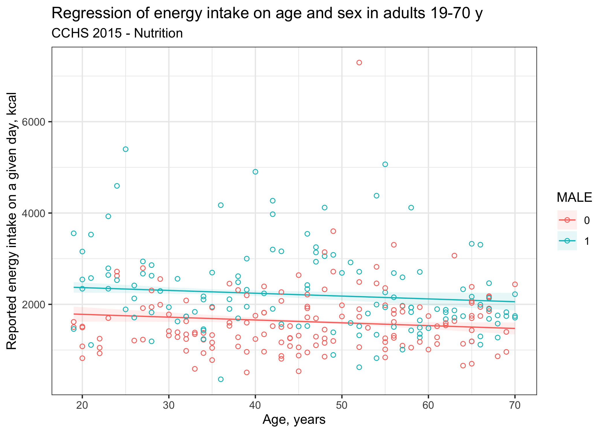
An important observation in the figure above is that “raw” energy intake values are not nicely centered around the regression curve, suggesting that our model does not fit the data very well. Energy intake reported on a given day is affected by substantial random errors, i.e., as much as 60%. In other words, the majority of the variance in (raw) energy intake on a given day is simply due to the fact that people eat more or less foods from day to day, which has not been accounted for in this analysis. Finally, one should also carefully check model assumptions (linearity, residuals normality, homoscedasticity) which I also did not show here for simplicity. Addressing non-linearity in linear regression models is a relevant topic for a future post.
Equivalent SAS code
I made a SAS code to reproduce the R analysis, which can be downloaded here.
References
Garriguet, D. 2018. “Accounting for Misreporting When Comparing Energy Intake Across Time in Canada.” Journal Article. Health Rep 29 (5): 3–12. https://www.ncbi.nlm.nih.gov/pubmed/29852052.
Health Canada. 2017. “Reference Guide to Understanding and Using the Data: 2015 Canadian Community Health Survey - Nutrition.” Government Document. https://www.canada.ca/en/health-canada/services/food-nutrition/food-nutrition-surveillance/health-nutrition-surveys/canadian-community-health-survey-cchs/reference-guide-understanding-using-data-2015.html.
Lumley, Thomas. 2010. “Complex Surveys,” February. https://doi.org/10.1002/9780470580066.
———. 2020. “Survey: Analysis of Complex Survey Samples.” https://rdocumentation.org/packages/survey/versions/4.1-1.