In medicine, epidemiology or nutrition, we measure data on features about the world we are interested in. It is often the case that we cannot obtain a perfect measure. For example, we cannot observe many people’s diet everyday over many months to determine usual dietary intakes. Instead, we use dietary assessment instruments to collect imperfect information about diet.

What does “imperfect” mean? Imperfect means there are expected differences between the variable we measured, e.g., as obtained with the dietary assessment instrument, and the variable we are interested in, e.g., true long-term dietary intakes. In other words, our measurements of diet have errors. Unfortunately, all dietary assessment instruments have errors (Thompson et al. 2015). However, it is useful to distinguish between two broad types of errors: random and systematic. As described in details elsewhere, “understanding the nature of that error can lead to better assessment, analysis, and interpretation of results” (Thompson et al. 2015). In this post, I aim to provide a simple demonstration of how random and systematic errors affect dietary assessment using simple simulation and R code.

Disclaimer: I have a PhD in nutrition, thus my knowledge of statistical methods is that of a naive enthusiast at best. I aim to provide a practical introduction based on my understanding. Please correct me where needed.

Understanding the difference between systematic and random

Definition

It is a bit challenging to give a simple definition without relying on other statistical concepts. A key difference is that we can mitigate random errors by collecting repeated measurements, but not systematic errors. A systematic error indicates that there will always be a difference compared with the truth. Thus, systematic errors are errors that cause a difference between the mean value and the true mean value, also known as bias. Random errors are errors that do not affect the average (mean) of a measurement, but only the measurement’s variability (or variance).

Systematic error example

Say we want to measure the consumption of vegetables and fruits in servings per day. We ask some individuals to self-report how many vegetables and fruits servings they ate on average per day during the last 4 weeks. We could imagine that the mean consumption of the vegetables and fruits affected by the systematic error is based on a self-reported measure obtained among a group of individuals with high social desirability (Hebert et al. 1995). Individuals could thus have overestimated their consumption of vegetables and fruit relative to their actual consumption, given that vegetables and fruit are more nutritious foods and that greater consumption is desirable.

# ********************************************** #
#             Load required packages             #
# ********************************************** #

library(dplyr)
library(ggplot2)
library(glue)

# Set theme for all plots
theme_set(ggplot2::theme_bw())

# ********************************************** #
#               Simple simulation                #
# ********************************************** #

set.seed(123)

# Set number of observations, mean, StdDev
  n <- 1000
  mean_value <- 5
  std <- 1
  bias <- 1
  
# Create variable consistent with values above
  x <- rnorm(n=n, mean=mean_value, sd=std)

# Create data without error, i.e., as it is
  sim_without <-
    data.frame(x = x , type = "accurate")

# Create systematic errors (i.e., errors that change the mean value or cause bias)
  systematic_errors <- rnorm(n=n, mean=bias, sd=0.1)
  
    # technical note: the sd=0.1 is very low relative to the standard deviation of x
    # to avoid adding random errors in this example

# Create data with error, i.e., with some bias
  sim_with <-
    data.frame(x = x + systematic_errors, ## add systematic errors to the accurately measured variable
               type="inaccurate")

# Combine both
  sim_data <-
    rbind(sim_without,sim_with)

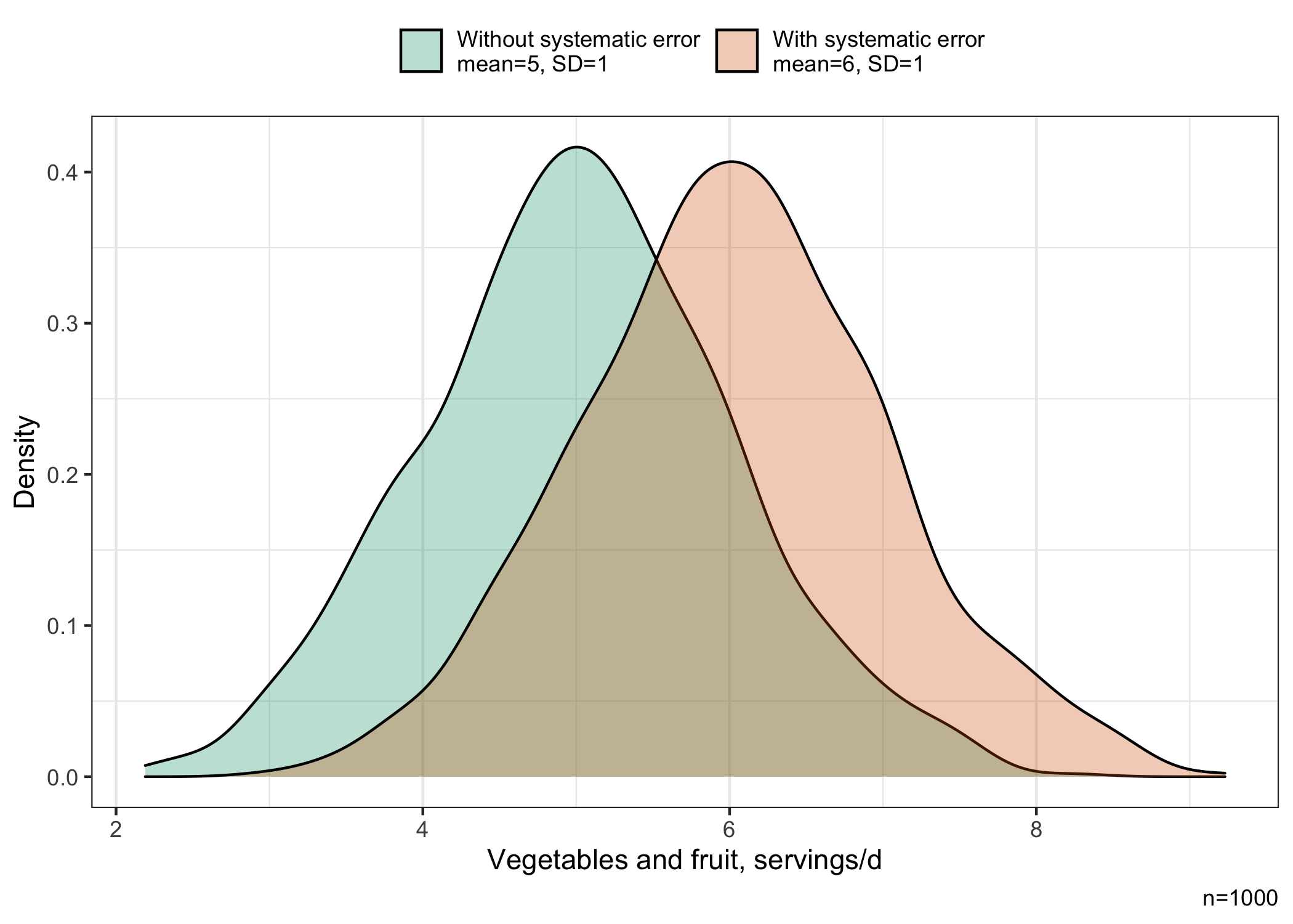
The simulated mean of the distribution of vegetable and fruit servings affected by the systematic error (6 servings/day) is higher than the mean of the unaffected distribution of vegetable and fruit servings (5 servings/day), while the standard deviation is approximately similar (1 serving/day).

# ********************************************** #
#               Show distributions               #
# ********************************************** #

# Color and label
color <-
  c("#009E73","#D55E00")

labeldistrib <-
  c( "accurate" =
       glue::glue("Without systematic error
                  mean={round(mean(sim_without$x),1)}, SD={round(sd(sim_without$x),1)}"), 
     "inaccurate"  =
       glue::glue("With systematic error
                  mean={round(mean(sim_with$x),1)}, SD={round(sd(sim_with$x),1)}")
     )

# Graph
  ggplot(data=sim_data,aes(x=x),color=type) +
  geom_density(aes(fill=type),alpha=0.3) +
  scale_fill_manual(name="Distribution",labels=(labeldistrib),values=color) +
  labs(y="Density",
       x="Vegetables and fruit, servings/d",
       caption=paste0("n=",n)
       ) +
    theme(panel.grid.major.y = element_blank(),
          legend.title = element_blank(),
          legend.position = "top")

Random error example

Say we also want to measure the consumption of vegetables and fruits. However, we use a different dietary assessment instrument this time: a short-term instrument assessing intakes on a given day. Perhaps we may prefer a short-term instrument to avoid relying on memory (e.g., using a 1-d food record) or to mitigate other source of bias (Freedman et al. 2014). However, there is a trade-off to this strategy: the dietary assessment no longer reflect dietary intakes over many days or weeks, but only intakes on a given day.

This matters because dietary intakes vary randomly from one day to another. On any given day, perhaps you may have eaten a little more (or a little less) than usual. The measurement of vegetables and fruits intake on a given day therefore reflects this random deviation from true intakes over a long period that we would have observed, had we been able to assess intakes over such period. In other words, while the short-term assessment on the dietary intakes on a given day is entirely accurate, it does not reflect the average intake over the long-term. Typically, long-term dietary intakes are what matters in term of adherence to recommendations, nutritional status and chronic disease risk reduction. For example, eating a ton of vegetables and fruits on a single occasion per year would not be sufficient to produce health benefits. Rather, it is the long-term, “usual” exposure to vegetables and fruits that is the most relevant.

# ********************************************** #
#               Simple simulation                #
# ********************************************** #

set.seed(123)

# Set number of observations, mean, StdDev
  n <- 1000
  mean_value <- 5
  std <- 1
  

# Create variable consistent with values above
  x <- rnorm(n=n, mean=mean_value, sd=std)
  
# Create data without random error, i.e., as it is
  sim_without <-
    data.frame(x = x, type = "precise")

# Create random errors (i.e., errors that only contribute to variability hence mean=0)
  random_errors <- rnorm(n=n, mean=0, sd=1.3)
  
  # technical note: because sd=1.3, random errors have a larger variance than the measurement.
  # This is however consistent with dietary intakes measured on a given day.

# Create data with random error, i.e., with some imprecision
  sim_with <- 
    data.frame(
      x = x + random_errors , ## errors added to the precisely measured values
               type="imprecise")

  ## Truncate any zero to reflect dietary intakes
  sim_with$x [sim_with$x < 0 ] <- 0

# Combine both
sim_data2 <-
  rbind(sim_without,sim_with)

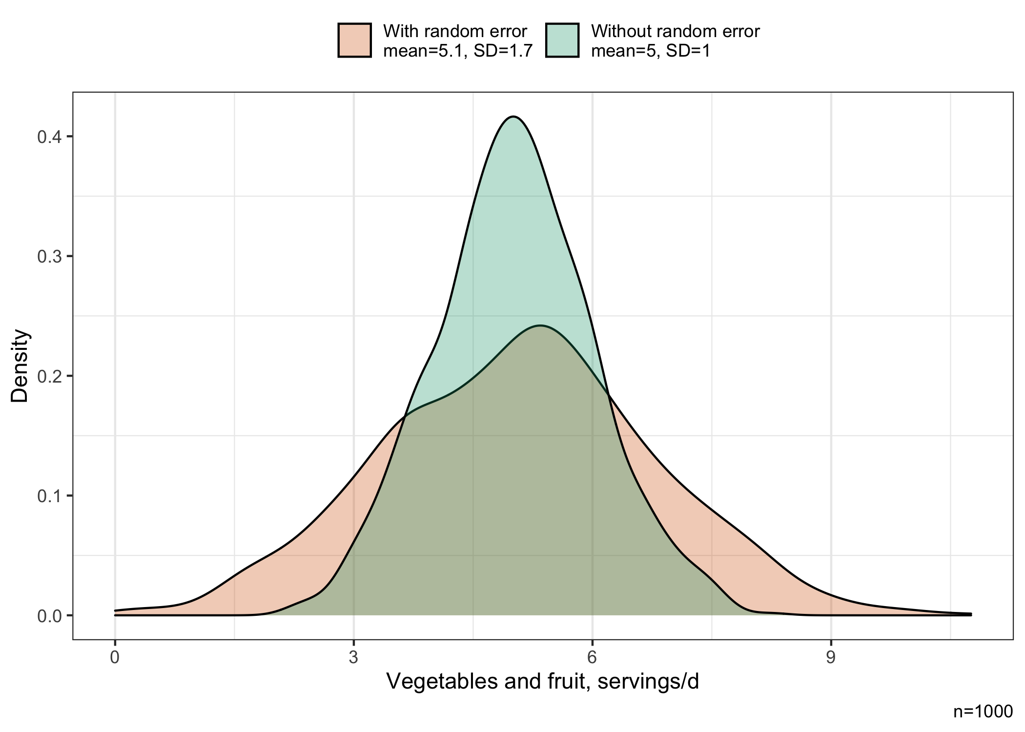
The standard deviation of the variable measured with random errors (1.7 servings/day) is larger than for the variable measured without random errors (1 serving/day), indicating greater variability around the mean. The means are approximately similar at 5.02 and 5.07 servings/day for the distribution measured without and with errors, respectively.
The distribution of vegetables and fruits is shown below. We see that the distribution measured with random errors is wider than the distribution measured without random errors, consistent with the greater variability around the mean.

# ********************************************** #
#               Show distributions               #
# ********************************************** #

# Color and label
color <-
  c("#D55E00","#009E73")

labeldistrib <- 
  c( "precise" =
       glue::glue("Without random error
                  mean={round(mean(sim_without$x),1)}, SD={round(sd(sim_without$x),1)}"), 
     "imprecise"  =
       glue::glue("With random error
                  mean={round(mean(sim_with$x),1)}, SD={round(sd(sim_with$x),1)}")
     )

# Graph
  ggplot(data=sim_data2,aes(x=x),color=type) +
  geom_density(aes(fill=type),alpha=0.3) +
  scale_fill_manual(name="Distribution",labels=(labeldistrib),values=color) +
  labs(y="Density",
       x="Vegetables and fruit, servings/d",
       caption=paste0("n=",n)
       ) +
    theme( panel.grid.major.y = element_blank(),
           legend.title = element_blank(),
           legend.position = "top")

Implications for nutrition research

“So what?” You might be thinking at this point. The knowledge of these errors in nutrition research is important for many reasons.

1. There are methods to mitigate random errors, but it is much more difficult to mitigate systematic errors. Thus, it is generally desirable to use a dietary assessment instrument that is the least affected by systematic errors. This is an area where we can improve study design by opting for an instrument less prone to bias, see (Thompson et al. 2015; Freedman et al. 2014) and the National Cancer Institute Dietary Assessment Primer.

2. Knowledge of the presence of random errors helps guide analyses (Keogh et al. 2020; Thompson et al. 2015). For example, it may be necessary (or not!) to account for the random errors depending on the research objective (Keogh et al. 2020; Dodd et al. 2006). The knowledge of errors therefore contribute to better analysis.

3. The interpretation of results is improved by knowledge of the inherent limitation of dietary assessment instruments. Indeed, even the “best” instrument have some degree of systematic error for example (Thompson et al. 2015; Freedman et al. 2014). Plus, random errors correction method are also based on the assumption that the diet measurement is otherwise unbiased (Kirkpatrick et al. 2022), which we know is not entirely true (Freedman et al. 2014). In other words, we must stay humble given the difficulty of the task!

In a future blog post, I will show the impact of random errors for different research objectives as well as how we can apply correction methods.

References

Dodd, K. W., P. M. Guenther, L. S. Freedman, A. F. Subar, V. Kipnis, D. Midthune, J. A. Tooze, and S. M. Krebs-Smith. 2006. “Statistical Methods for Estimating Usual Intake of Nutrients and Foods: A Review of the Theory.” Journal Article. J Am Diet Assoc 106 (10): 1640–50. https://doi.org/10.1016/j.jada.2006.07.011.

Freedman, L. S., J. M. Commins, J. E. Moler, L. Arab, D. J. Baer, V. Kipnis, D. Midthune, et al. 2014. “Pooled Results from 5 Validation Studies of Dietary Self-Report Instruments Using Recovery Biomarkers for Energy and Protein Intake.” Journal Article. Am J Epidemiol 180 (2): 172–88. https://doi.org/10.1093/aje/kwu116.

Hebert, J. R., L. Clemow, L. Pbert, I. S. Ockene, and J. K. Ockene. 1995. “Social Desirability Bias in Dietary Self-Report May Compromise the Validity of Dietary Intake Measures.” Journal Article. Int J Epidemiol 24 (2): 389–98. https://www.ncbi.nlm.nih.gov/pubmed/7635601.

Keogh, R. H., P. A. Shaw, P. Gustafson, R. J. Carroll, V. Deffner, K. W. Dodd, H. Kuchenhoff, et al. 2020. “STRATOS Guidance Document on Measurement Error and Misclassification of Variables in Observational Epidemiology: Part 1-Basic Theory and Simple Methods of Adjustment.” Journal Article. Stat Med 39 (16): 2197–2231. https://doi.org/10.1002/sim.8532.

Kirkpatrick, S. I., P. M. Guenther, A. F. Subar, S. M. Krebs-Smith, K. A. Herrick, L. S. Freedman, and K. W. Dodd. 2022. “Using Short-Term Dietary Intake Data to Address Research Questions Related to Usual Dietary Intake Among Populations and Subpopulations: Assumptions, Statistical Techniques, and Considerations.” Journal Article. J Acad Nutr Diet. https://doi.org/10.1016/j.jand.2022.03.010.

Thompson, Frances E., Sharon I. Kirkpatrick, Amy F. Subar, Jill Reedy, TusaRebecca E. Schap, Magdalena M. Wilson, and Susan M. Krebs-Smith. 2015. “The National Cancer Institute’s Dietary Assessment Primer: A Resource for Diet Research.” Journal of the Academy of Nutrition and Dietetics 115 (12): 1986–95. https://doi.org/10.1016/j.jand.2015.08.016.