
Impact of random errors: two nutrition examples
Published:
In my previous blog, I explained the difference between systematic and random errors. While it is obvious that a systematic error (difference) between the “true” value and its measurement can be a problem, the impact of random errors is often more subtle. However, in many cases, random errors can be as problematic as systematic errors if they are ignored. In this post, I aim to provide a simple demonstration of how random errors may cause problems for two common analyses in nutrition.
The first example is a surveillance-type analysis, where the research question aims at estimating the proportion of individuals above or below a cut-off. The second example is an epidemiological-type analysis, where the research question aims at estimating the association between diet, as independent variable, and an outcome.
Disclaimer: I have a PhD in nutrition, thus my knowledge of statistical methods is that of a naive enthusiast at best. I aim to provide a practical introduction based on my understanding. Please correct me where needed.

Example 1: distribution of a single variable measured with errors
A hypothetical study objective could be to estimate the proportion of individuals with low vegetables and fruits intake (\(X\)), say less than 4 servings per day. The target statistics of interest (or estimand) is \(Pr(X<4)\). To measure vegetables and fruits intake, we could use the 24-h dietary recall which provides 1-day worth of intake data with minimal systematic error (Thompson et al. 2015). However, we know that intakes on a given day may differ from the long-term average or usual vegetables and fruits intake (Dodd et al. 2006). The measurement of vegetables and fruits intake (\(W\)) with a 24-h dietary recall is affected by random errors.
Simulation
In the code below, I show a simple simulation to obtain data consistent with the example described.
# ********************************************** #
# Prepare simulated measures #
# ********************************************** #
set.seed(1)
# generate the 'true' value (no random errors)
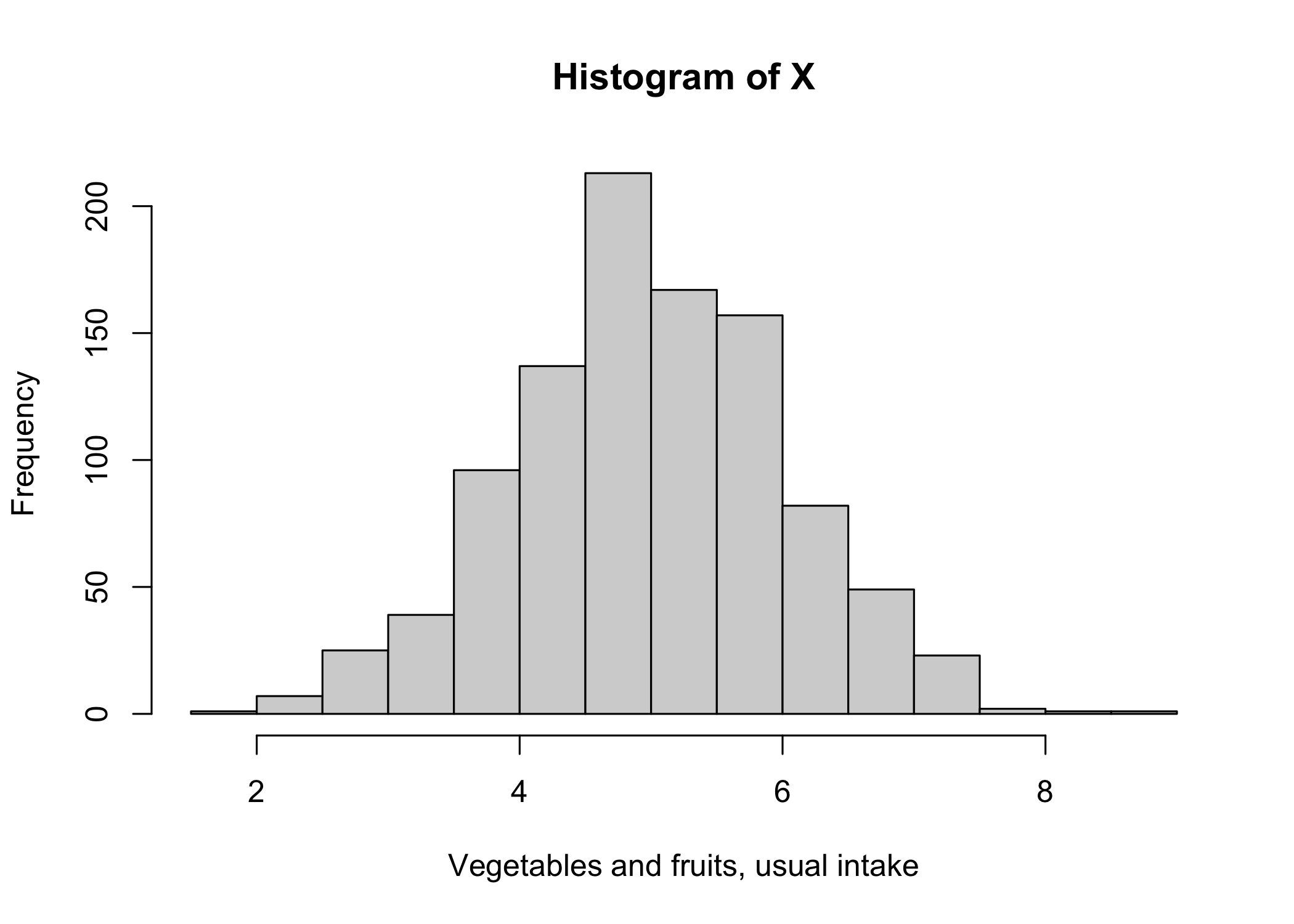
X <- rnorm(n=1000, mean=5, sd=1)
hist(X,xlab="Vegetables and fruits, usual intake")
  # generate random errors
  E1 <- rnorm(n=1000, mean=0, sd=1.3)

  # combine the 'true' value with random errors to derive the measured value (X "on a given day")
  W1 <- X+E1

    ## For plausibility, truncate negative values at 0 (i.e., cant have negative intakes)
    W1 <- ifelse(W1<0,0,W1)

  hist(W1,xlab="Vegetables and fruits, on a given day")
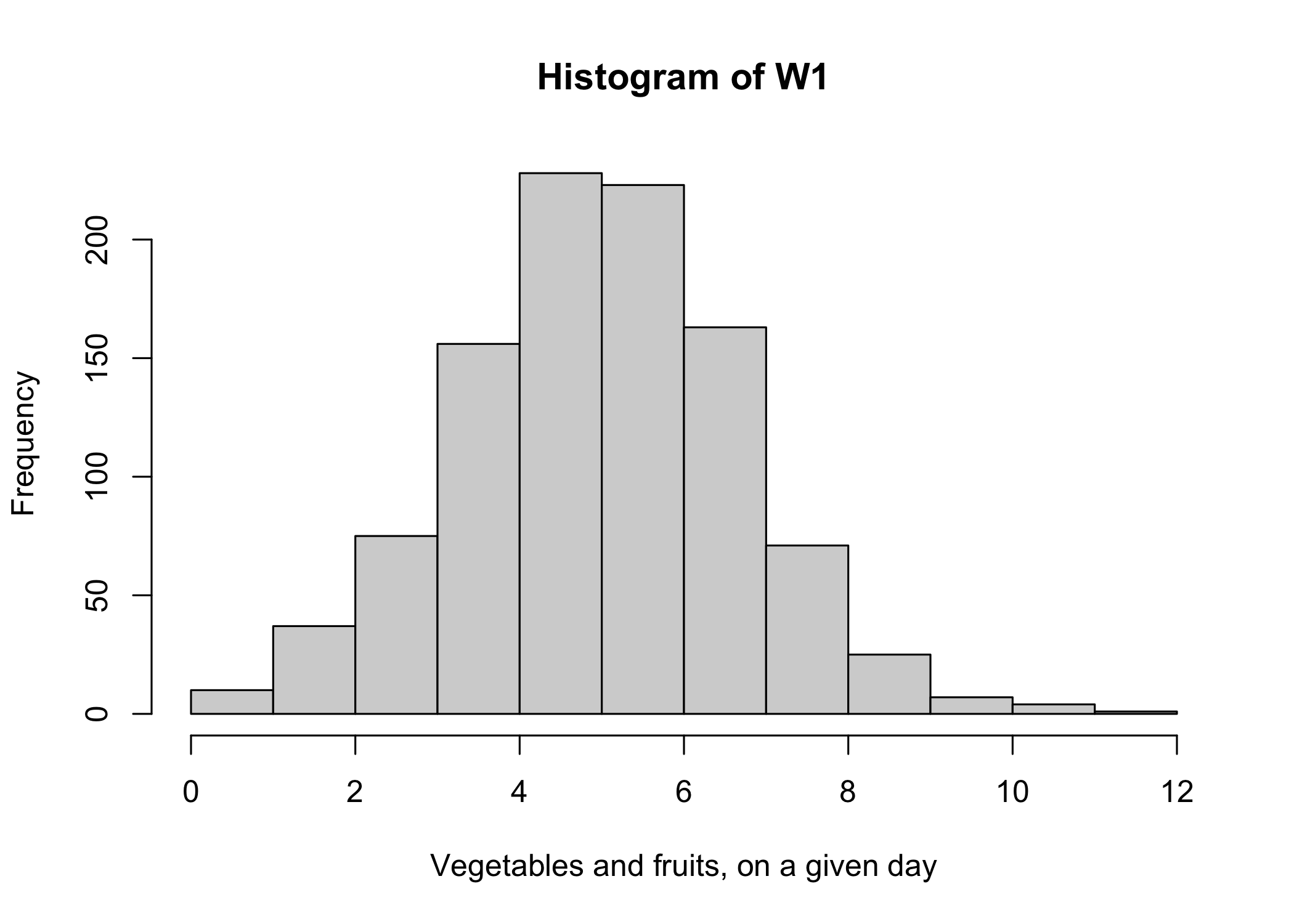
First, the good news! By definition, the mean of the vegetables and fruits intakes measured with random errors (\(\mu_{W_1}\)= 4.97) is approximately the same as the mean of the “true” intakes without errors (\(\mu_{X}\)= 4.99). So, if the objective of the analysis is to estimate the mean of a single variable measured with random errors, we could safely ignore random errors. The estimate of the mean would be correct! Now, the bad news…
Proportion of individuals above or below a cut-off
# ********************************************** #
#        Calculate proportions < cut-off         #
# ********************************************** #

# indicate value
cutoff <- 4

# Based on measured vegetables and fruits on a given day (i.e., 1x 24-h recall)
table(W1<cutoff)/1000
FALSE  TRUE
0.722 0.278
# Based on "true" vegetables and fruits consumption (i.e., long-term or usual average)
table(X<cutoff)/1000
FALSE  TRUE
0.832 0.168
A naive analysis ignoring random errors would use the measured intakes of vegetables and fruits on a given day (a single 24-h dietary recall) to estimate the proportion of individuals below the 4 servings per day cut-off. Such analysis would show that there are 28% of the sample with intakes <4 servings/day (\(Pr(W_1<4)=\) 28%). However, had we been able to observe or assess “true” intakes, we would have found that only 17% of the sample actually had intakes <4 servings/day (\(Pr(X<4)=\) 17%). This is a difference of 11 percentage point!
The figure below illustrates the problem of considering intakes on a given day as if they were the same as usual or long-term intakes.
Visualization and Interpretation
# ********************************************** #
#           Prepare Distribution Data            #
# ********************************************** #

# <univariate_distrib> function
univariate_distrib <-
  function (x) {
distrib <-
data.frame(
  value=quantile(x,seq(1,99)/100, type=2)
)
distrib$p <- seq.int(1:99)
return(distrib[,2:1])
}

# estimate distribution
distrib_X <-  univariate_distrib(X) |> dplyr::mutate(name="X")
distrib_W1 <-  univariate_distrib(W1) |> dplyr::mutate(name="W1")

# append both
distrib_both <-
  rbind(distrib_X, distrib_W1)

## Add labels
distrib_both$name_f <-
  factor(distrib_both$name,
         levels = c("X","W1"),
         labels = c("Usual","Day 1"))


# ********************************************** #
#     Generate Cumulative Distribution Plot      #
# ********************************************** #

library(dplyr)
library(ggplot2)

# define color (usual, given day)
distrib_colors <- c("#788f33","#bf3626")

distrib_both |>
  ggplot(aes(x=value,y=p,color=name_f)) +
  geom_line(aes(linetype=name_f,colour=name_f),size=1.4) +
  geom_vline(xintercept=4,linetype=2,color="gray")+
  # id curve on a given day (W1)
  annotate(
    geom = "curve",
    x = 7.5, y = 85,
    xend = 7.5, yend = with(distrib_both|>filter(name=="W1"), which.min(abs(value - 7.5)))-2,
    curvature = -.3, arrow = arrow(length = unit(2, "mm")) ) +
  annotate(geom = "text", x = 7.5, y = 85, label = "On a given day",hjust = "right") +
  # id curve usual (X)
    annotate(
      geom = "curve", x = 5, y = 75,
      xend = 5.5, yend = with(distrib_both|>filter(name=="X"), which.min(abs(value - 5.5)))+2,
      curvature = -.3, arrow = arrow(length = unit(2, "mm")) ) +
    annotate(geom = "text", x = 5, y = 75, label = "Usual ('true')", hjust = "left") +
  # Cut-off value
  annotate(geom = "text", x =4, y = 90,
           label = "Pr(X<4)", vjust=1.5,size = 4 ) +
  # line colours
  scale_colour_manual(name="Distribution",
                      values = distrib_colors )+
  scale_linetype(name="Distribution") +
  labs(title="Cumulative distributions",
       x="Servings/day",y="Percentile") +
  scale_x_continuous(breaks=seq(2,10,2))+
  coord_flip() +
  theme_bw() +
  theme(legend.position="none",
        panel.grid.minor.y = element_blank()
        )
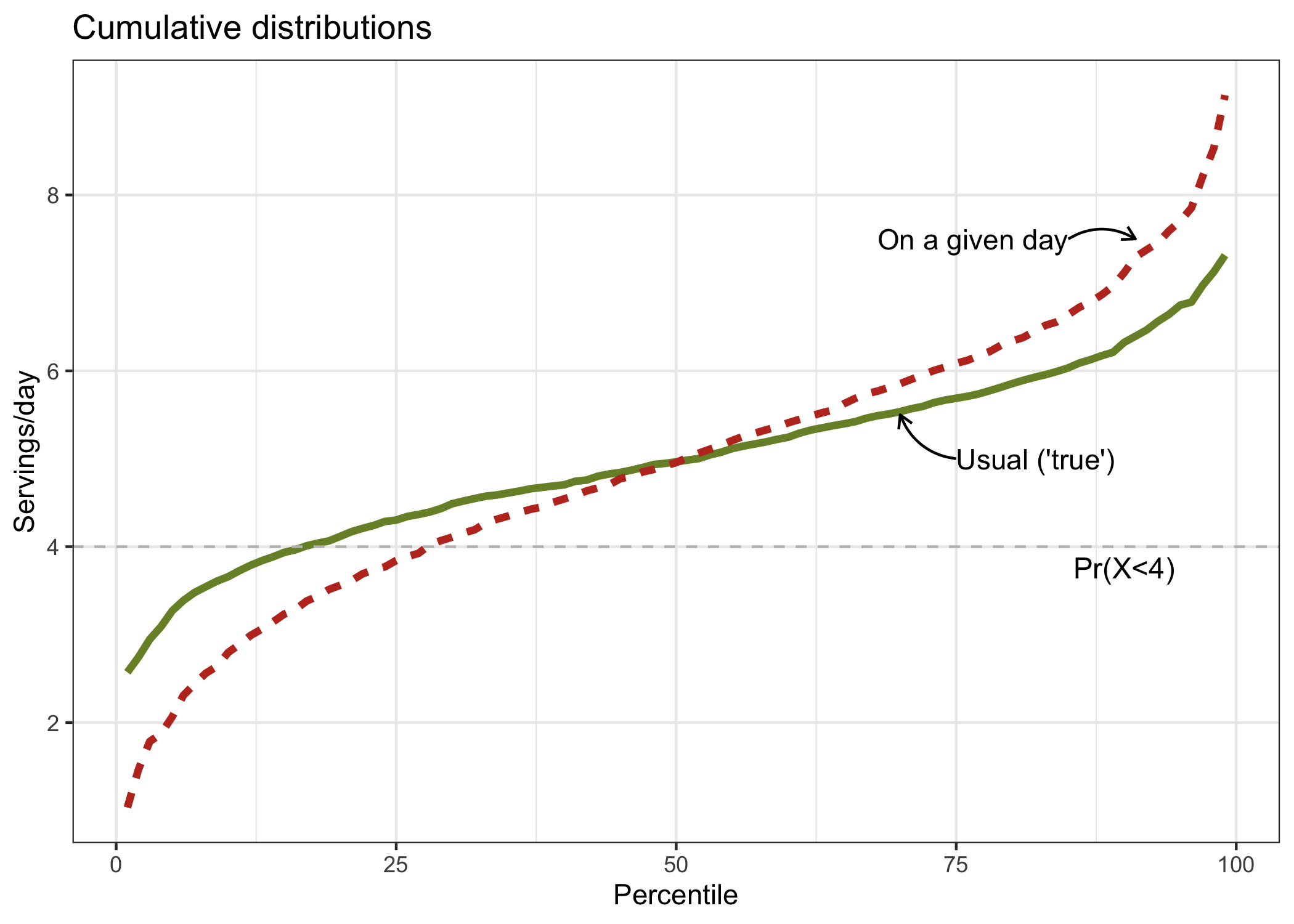
In the figure, we see that for lower percentiles (below 50th), the percentile estimates of vegetables and fruits intakes on a given day are underestimated as they fall below the “true” percentile estimates. Accordingly, the proportion of the sample with intakes below 4 servings per day is overestimated. In other words, random errors falsely inflates our estimate. In this example, one could incorrectly conclude that a substantial proportion of individuals have low intakes of vegetables and fruits, which would not be entirely consistent with the true estimate. In nutrition, this happens because there are always some individuals that ate more or less than usual on any given day for random reasons.
Of note, had we decided to estimate the proportion of the sample with high vegetables and fruits intake, say >6 servings per day, random errors would have caused similar problems. For higher percentiles (above 50th), the percentile estimates of vegetables and fruits intakes on a given day are overestimated as they fall above the “true” percentile estimates.
Example 2: relationship between one (1) independent variable measured with errors and an outcome
Another common study objective is to estimate the relationship between a dietary factor, as independent variable, and an outcome, as dependent variable. For a continuous outcome, the estimand is \(E(Y|X)\) or the expected value of \(Y\) given \(X\). For such analysis, we could be interested in the relationship between intake of vegetables and fruits (servings/day) and low-density lipoproteins (LDL) cholesterol concentrations as outcome; an association was found previously (Djousse et al. 2004). In other words, we want to estimate the expected LDL cholesterol concentrations based on the intake of vegetables and fruits in a sample of the population.
We could measure vegetables and fruits intake with 24-h dietary recall data since this instrument has minimal systematic error (Thompson et al. 2015). Of note, I assume that LDL cholesterol concentrations are measured perfectly and that there is no source of bias (no confounding, no selection bias, no differential errors,…). To assess such relationship, we could use a linear regression model corresponding to
\[Y_i=\beta_0 + \beta_{X_i} X_i +\epsilon_i\]A naive analysis ignoring random errors would rather have the estimand \(E(Y|W_1)\) and model equation:
\[Y_i=\beta\prime_0 + \beta\prime_{W_i} W_i +\epsilon_i\]Simulation
In this simulation, each increase of 1 serving of vegetables and fruits will decrease LDL cholesterol concentrations by 0.10 mmol/L. This is the true regression coefficient \(\beta_{X}\) for this association.
# ********************************************** #
#           Prepare simulated measures           #
# ********************************************** #

set.seed(1)
  # generate the 'true' value (no random errors)
  X  <- rnorm(n=1000, mean=5, sd=1)

  # generate random errors
  E1 <- rnorm(n=1000, mean=0, sd=1.3)

  # combine the 'true' value with random errors to derive the measured value (X "on a given day")
  W1 <- X+E1

    ## For plausibility, truncate negative values at 0 (i.e., cant have negative intakes)
    W1 <- ifelse(W1<0,0,W1)

  # generate a linear relationship based on X
  b0 <- 3.0 # hypothetical average LDL cholesterol in this sample
  b1 <- -0.10 # hypothetical relationship between vegetables and fruits and cholesterol
  EQ <-  b0 + b1 * X
  Y  <-  rnorm(n=1000, EQ, sd=0.5)
Relationship based on linear regression models
First, I assess the relationship based on the naive analysis which considers the measured vegetables and fruits on a given day as if it reflected long-term/usual intakes. Then, I repeat the analysis by using the true value, i.e., vegetables and fruits intake measured without errors that reflects long-term/usual intakes.
# ********************************************** #
#        Association for naive analysis          #
# ********************************************** #

# Model for E(Y|W)
naive <- lm(Y ~ W1)

# Model parameters
naive_param <-
  parameters::model_parameters(naive)

naive_param
Parameter   | Coefficient |       SE |         95% CI | t(998) |      p
-----------------------------------------------------------------------
(Intercept) |        2.62 |     0.05 | [ 2.52,  2.72] |  51.80 | < .001
W1          |       -0.02 | 9.63e-03 | [-0.04,  0.00] |  -2.35 | 0.019
# ********************************************** #
#                True association                #
# ********************************************** #

# Model for E(Y|X)
true <- lm(Y ~ X)

# Model parameters
true_param <-
  parameters::model_parameters(true)

true_param
Parameter   | Coefficient |   SE |         95% CI | t(998) |      p
-------------------------------------------------------------------
(Intercept) |        2.88 | 0.08 | [ 2.73,  3.04] |  35.96 | < .001
X           |       -0.08 | 0.02 | [-0.11, -0.04] |  -4.79 | < .001
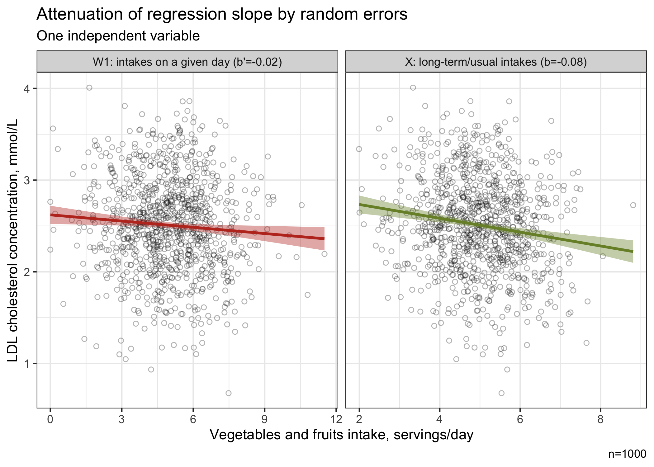
The naive analysis indicates that a 1-serving increase in vegetables and fruits is associated with a 0.02 mmol/L lower LDL cholesterol concentrations (95%CI, -0.04, 0.00). However, the analysis based on “true” intakes rather indicates that a 1-serving increase in vegetables and fruits is associated with a 0.08 mmol/L lower LDL cholesterol concentrations (95%CI, -0.11, -0.04), consistent with the “true” simulated association. The naive analysis shows a 3.3-fold attenuation of the true relationship!
Visualization and Interpretation
In this example, ignoring random errors could affect our conclusion. Indeed, based on the naive analysis which ignores random errors, we may be tempted to conclude that the association between vegetables and fruits and LDL cholesterol is not clinically relevant. However, we get a different picture when the association is estimated based on “true” vegetables and fruits intake, a measure that is not affected by random errors.
The figure below shows that the regression curve based on the intake of vegetables and fruits on a given day (with random error) is attenuated compared with the curve based the true intake of vegetables and fruits which reflects long-term/usual consumption.
library(dplyr)
library(ggplot2)

# ********************************************** #
#  Regression curve for true and naive analysis  #
# ********************************************** #

# combine simulation data
model_data <-
  tibble::tibble(
    X=X,
    W1=W1,
    Y=Y) |>
  tidyr::pivot_longer(cols=c(X,W1),
                      names_to="Measure",
                      values_to="VF_intake")

# define color (on a given day, usual)
curve_colors <- c("#bf3626","#788f33")

# define labels
curve_labels <-
  c("W1" = paste0("W1: intakes on a given day (b'=",round(naive_param[2,"Coefficient"],2),")"),
    "X" = paste0("X: long-term/usual intakes (b=",round(true_param[2,"Coefficient"],2),")"))

# plot of regression curves side by side
  ggplot(data=model_data,aes(x = VF_intake, y = Y,group=Measure)) +
  geom_point(shape=1,alpha = 0.3) +
  geom_smooth(method = "lm",aes(color=Measure,fill=Measure)) +
  facet_wrap(~Measure,scales="free_x",labeller=as_labeller(curve_labels)) +
    scale_color_manual(values=curve_colors) +
    scale_fill_manual(values=curve_colors) +
  labs(title = "Attenuation of regression slope by random errors",
       subtitle = "One independent variable",
       x="Vegetables and fruits intake, servings/day",y="LDL cholesterol concentration, mmol/L",
       caption="n=1000") +
  theme_bw() +
  theme( legend.position = "none"
  )
Of note, random errors do not always cause attenuation (Brakenhoff et al. 2018; Smeden, Lash, and Groenwold 2020)! The impact varies depending on whether the variable measured with errors is the independent or not; or according to the number of independent variable(s) measured with random errors among others.
Conclusion
These simple examples are a simplified version of reality. Sometimes, we have access to repeated 24-h dietary recalls which could mitigate, to some extent, the problems associated with random errors. Nonetheless, it is useful to know when measurement error correction methods should be used for optimal results that are closer to the truth!
Useful references to learn more about these issues include a thorough review by Keogh et al. (2020). Brakenhoff et al. (2018) also shows the impact of random errors on regression coefficient when two independent variables measured with errors are included in a model. In a future post, I will show how we can apply measurement error correction method to mitigate the negative impact of random errors.
References
Brakenhoff, T. B., M. van Smeden, F. L. J. Visseren, and R. H. H. Groenwold. 2018. “Random Measurement Error: Why Worry? An Example of Cardiovascular Risk Factors.” Journal Article. PLoS One 13 (2): e0192298. https://doi.org/10.1371/journal.pone.0192298.
Djousse, L., D. K. Arnett, H. Coon, M. A. Province, L. L. Moore, and R. C. Ellison. 2004. “Fruit and Vegetable Consumption and LDL Cholesterol: The National Heart, Lung, and Blood Institute Family Heart Study.” Journal Article. Am J Clin Nutr 79 (2): 213–17. https://doi.org/10.1093/ajcn/79.2.213.
Dodd, K. W., P. M. Guenther, L. S. Freedman, A. F. Subar, V. Kipnis, D. Midthune, J. A. Tooze, and S. M. Krebs-Smith. 2006. “Statistical Methods for Estimating Usual Intake of Nutrients and Foods: A Review of the Theory.” Journal Article. J Am Diet Assoc 106 (10): 1640–50. https://doi.org/10.1016/j.jada.2006.07.011.
Keogh, R. H., P. A. Shaw, P. Gustafson, R. J. Carroll, V. Deffner, K. W. Dodd, H. Kuchenhoff, et al. 2020. “STRATOS Guidance Document on Measurement Error and Misclassification of Variables in Observational Epidemiology: Part 1-Basic Theory and Simple Methods of Adjustment.” Journal Article. Stat Med 39 (16): 2197–2231. https://doi.org/10.1002/sim.8532.
Smeden, M. van, T. L. Lash, and R. H. H. Groenwold. 2020. “Reflection on Modern Methods: Five Myths about Measurement Error in Epidemiological Research.” Journal Article. Int J Epidemiol 49 (1): 338–47. https://doi.org/10.1093/ije/dyz251.
Thompson, Frances E., Sharon I. Kirkpatrick, Amy F. Subar, Jill Reedy, TusaRebecca E. Schap, Magdalena M. Wilson, and Susan M. Krebs-Smith. 2015. “The National Cancer Institute’s Dietary Assessment Primer: A Resource for Diet Research.” Journal of the Academy of Nutrition and Dietetics 115 (12): 1986–95.https://doi.org/10.1016/j.jand.2015.08.016.