
Analyzing the Canadian Community Health Survey (CCHS) 2015 data with R: mean diet quality score
Published:
In a previous post, I showed how to account for the Canadian Community Health Survey (CCHS) complex survey design for a simple analysis in R. However, some nutrition analyses require multiple steps that are not “built-in” in a statistical software. For example, the recommended approach to estimate a (mean) diet quality score based on 24-hour dietary recall data, the main dietary assessment instrument in surveys, is the population ratio method (Freedman et al. 2008).
The goal of this post is to provide R code showing how to account for the CCHS 2015 design to calculate a diet quality score using the population ratio method. Note that data for the CCHS 2015 - Nutrition (Public Use Micro Datafile or PUMF) are publicly available.
Population ratio vs. simple scoring
Briefly, to derive a diet quality score using the population ratio method, dietary intakes and ratio of intakes are estimated at the population- or group-level then scored. For example, to score the percentage of total energy intake (%E) as saturated fats (SFA):
- we calculate the mean calories from saturated fats (\(\mu_{SFA}\)) and mean total energy intake in calories (\(\mu_{E}\)) in the overall population or group of interest.
- we divide the mean calories from saturated fat by the mean total energy intake \(\frac{\mu_{SFA}}{\mu_{E}}\).
- we apply the scoring algorithm, e.g., \(f(\frac{\mu_{SFA}}{\mu_{E}})\), to derive the diet quality score .
Alternatively, one could have used a simple scoring method In a simple scoring method, the scoring algorithm is directly applied to each respondent’s dietary intakes \(f(\frac{SFA_i}{E_i})\). Each respondent has a score and the mean of these scores is then used to estimate the mean diet quality score of the population or group: \(\mu_{f(\frac{SFA_i}{E_i})}\). Unfortunately, the simple scoring method is less optimal since it assumes that each respondent’s dietary intakes reflect usual dietary intakes, i.e., a long-term average. This is not the case when using only one 24-h dietary intake, because of random errors (more details here). Of note, the main issue in this example is that we apply a scoring to the dietary intakes and the “input” matters because scoring ‘truncates’ a distribution of intakes at certain cut-points. On the contrary, the population ratio method directly scores usual dietary intakes because mean intakes at the group level do reflect usual dietary intakes.
Example summary
Mean score according to the population ratio method:
\[\mu_{Score} = f(x) = f(\frac{\mu_{SFA}}{\mu_{E}})\]Mean score according to the simple scoring method:
\[\mu_{Score} = \mu_{f(x)} = \mu_{f(\frac{SFA_i}{E_i})}\]To obtain a mean diet quality score, the population ratio method is more optimal since the scoring is applied to intakes that reflect long-term intakes rather than intakes on a given day.
Data preparation and overview
For demonstration purpose, I show how to calculate Healthy Eating Food Index (HEFI)-2019 scores according to smoking status (smokers vs. non-smokers as well as score difference). The HEFI-2019 is a continuous score that reflects the degree of adherence to Canada’s Food Guide 2019 recommendations on healthy food choices (Brassard et al. 2022a, b). The data used for the present example are already “pre-processed”. Complete details are shown in the HEFI-2019 Github repository.
# ********************************************** #
#             Load required packages             #
# ********************************************** #

library(tidyverse)
library(dplyr)
library(data.table)
library(parallel)
library(furrr)
library(ggplot2)
library(haven)

# HEFI-2019 scoring algorithm
  #if not installed, run: devtools::install_github("didierbrassard/hefi2019")
  library(hefi2019)

# ********************************************** #
#           Load and prepare CCHS data           #
# ********************************************** #

# 1) Load processed data, dietary intakes +  sociodemographic characteristics
  load(file.path("post_data","intake_per24hr.rdata"))
  load(file.path("post_data","hs_nci.rdata"))

# 2) Combine dietary intakes of the first recall with sociodemographic data

  intake_and_sociodeom <-
    inner_join(intake_per24hr,hs_nci|>select(ADM_RNO,SUPPID,WTS_P,drig,sex,age,smoking)) |>
    # remove 24-h recall with 0 energy intake & first 24-hr only & aged 19 y +
    filter(energy>0 & SUPPID==1 & age>=19) |>
    mutate(
      # recode smoking as yes or no
      smoking = ifelse(smoking %in% c(1,2),1,smoking)
    )

  #note: sample size of respondents 2y+ for first 24-h recall = 20,103

# 3) Load and prepare bootstrap replicate weights

  # Note: a hardcoded path (<external_drive>) is used since files are on an external drive.
  # Usually we would want analysis to be self-contained, but survey files are a bit large.
  # Also, the data are set-up exactly as they are once obtained from Statistics Canada

  bsw <-
    data.table::fread(file.path(external_drive,"CCHS_Nutrition_2015_PUMF","Bootstrap",
                                "Data_Donnee","b5.txt"),
                      stringsAsFactors = F, data.table= F, header=F,
                      col.names = c("ADM_RNO","WTS_P",paste0("BSW",seq(1,500)))) |>
    # keep only respondents in <intake_and_sociodeom>
    right_join(intake_and_sociodeom[,"ADM_RNO"]) |>
    # rename sampling weights
    rename(BSW0=WTS_P)

 # cchs_data overview
 head(intake_and_sociodeom)
# A tibble: 6 × 24
  ADM_RNO SUPPID    wg    rg  pfab  pfpb otherfoods    vf water otherbevs  milk
    <dbl>  <dbl> <dbl> <dbl> <dbl> <dbl>      <dbl> <dbl> <dbl>     <dbl> <dbl>
1       1      1 1.05   0.9  1.20   5.84      45.1  0     1917.        0    0
2       2      1 0      1.24 4.45   0         12.3  2.21     0      2125.   0
3       3      1 1.19   0    3.27   0          2.40 0.494  813.        0  122.
4       4      1 0.477  1.45 1.08   0          3.27 2.11  1873.      685.  11.4
5       5      1 0      0.96 1.74   6.45      74.1  6.96  2226.      391.  61.0
6       6      1 0      1.07 0.540  0          1.24 4.04  4129.      513.   0
# ℹ 13 more variables: plantbev <dbl>, freesugars <dbl>, energy <dbl>,
#   sfa <dbl>, mufa <dbl>, pufa <dbl>, sodium <dbl>, nonzero_energy <dbl>,
#   WTS_P <dbl>, drig <dbl>, sex <dbl>, age <dbl>, smoking <dbl>
 # bootstrap weight overview
 head(bsw[,1:6])
  ADM_RNO BSW0 BSW1 BSW2 BSW3 BSW4
1       1  859   31   33 2234   27
2       2  901  539   62   64   60
3       3 4431   41 5898 5498 8455
4       4  539   50   33   42 1941
5       5  703   50 1812   64   60
6       6   42  312  188  144  225
‘Population ratio’ function
Typically, we would use built-in function or package (e.g., the survey package in R) to obtain estimates and confidence interval. However, there is rarely a built-in function for multistage analyses. In the present case, there are different approaches to estimate variance of population ratio means with survey data. Perhaps the simplest approach - although not the most efficient - is to iteratively loop the analysis through all bootstrap replicate weights. In other words, we calculate mean estimates for each bootstrap weight and then calculate confidence intervals based on the (bootstrap) sampling distribution.
Since we will repeat the analysis 500+1 times to have diet quality score estimates for each bootstrap replicate weight as well as the original sampling weight, we create a function that will generate the desired statistics. This process will effectively account for the complex survey design and allow us to derive mean and difference.
# ********************************************** #
#      Function of mean, score, difference       #
# ********************************************** #

  # note: 'ADM_RNO', 'smoking' and  'hefi2019_vars' are hardcoded in this function and
  # should be modified if used for a different analysis.

  mean_score_diff <-
    function(bsw_number,indata,inbsw,bsw_suffix="BSW"){
    # Parameters:
      # bsw_number = number from 0 to 500 where 0 = original estimate and 1, 2, 3 ... 500 = bsw
      # indata = input data set
      # inbsw  = data set with bootstrap replicate weight
      # bsw_suffix = common suffix to all variables representing sampling and bootstrap weights

    # 1) Create weights variable
      weights <- paste0(bsw_suffix,bsw_number)

    # 2) calculate MEAN
      suppressMessages(
      estimate <-
        # combine weight value with indata
        dplyr::left_join(indata,inbsw |> select(ADM_RNO,!!weights)) |>
        # rename weights for use with weighted.mean
        dplyr::rename(CURRENT_BSW= !!weights ) |>
        # remove missing values
        dplyr::filter(is.na(smoking)==FALSE) |>
        # group by smoking status
        dplyr::group_by(smoking) |>
        # calculate weighted mean
        dplyr::summarise(
          across(.cols=all_of(hefi2019_vars),
                 function(x) weighted.mean(x,w=CURRENT_BSW),
                 .names ="{col}_MEAN" )
          # note: suffix <_MEAN> added for labeling population-level values (vs. respondent-level)
          ) |>
      # 3) SCORE: Apply the HEFI-2019 scoring algorithm to obtain
        hefi2019::hefi2019(#indata             = .,
          vegfruits          = vf_MEAN,
          wholegrfoods       = wg_MEAN,
          nonwholegrfoods    = rg_MEAN,
          profoodsanimal     = pfab_MEAN,
          profoodsplant      = pfpb_MEAN,
          otherfoods         = otherfoods_MEAN,
          waterhealthybev    = water_MEAN,
          unsweetmilk        = milk_MEAN,
          unsweetplantbevpro = plantbev_MEAN,
          otherbeverages     = otherbevs_MEAN ,
          mufat              = mufa_MEAN ,
          pufat              = pufa_MEAN ,
          satfat             = sfa_MEAN ,
          freesugars         = freesugars_MEAN,
          sodium             = sodium_MEAN,
          energy             = energy_MEAN)
      ) # end of suppress message

      # 3) DIFFERENCE: Calculate difference in smokers vs. non-smokers
      estimate_diff <-
        estimate |>
        dplyr::select(smoking,starts_with("HEFI")) |>
        tidyr::pivot_longer(
          cols = starts_with("HEFI"),
          names_to = "HEFI2019_components"
        ) |>
        tidyr::pivot_wider(
          names_from = "smoking",
          names_prefix = "SMK_"
        ) |>
        dplyr::mutate(
          DIFF = SMK_1 - SMK_0,
          # add BSW id
          replicate = bsw_number
        )
      # 4) remove temporary data and return final data with all statistics
      rm(estimate)
      rm(weights)
      return(estimate_diff)
    }
Calculate estimates with sampling weights
It is often best to verify that everything works as intended before running lengthy bootstrap analyses. For this test, we will estimate HEFI-2019 score based on the sampling weights (i.e., renamed from WTS_P to BSW0) without variance estimation.
# ********************************************** #
#        Run <mean_score_diff> with BSW0         #
# ********************************************** #

# 1) Define vectors of HEFI-2019 dietary constituents

  hefi2019_vars <- names(intake_per24hr[,3:(ncol(intake_per24hr)-1)])

  hefi2019_vars
 [1] "wg"         "rg"         "pfab"       "pfpb"       "otherfoods"
 [6] "vf"         "water"      "otherbevs"  "milk"       "plantbev"
[11] "freesugars" "energy"     "sfa"        "mufa"       "pufa"
[16] "sodium"
  # note: this works since the <intake_per24hr> was specifically created to calculate HEFI-2019 scores.

# 2) Apply function

 popratio_hefi2019_bsw0 <-
    mean_score_diff(bsw_number = 0,
              indata = intake_and_sociodeom,
              inbsw  = bsw)

 # 3) Show output

 popratio_hefi2019_bsw0
# A tibble: 11 × 5
   HEFI2019_components   SMK_0  SMK_1   DIFF replicate
   <chr>                 <dbl>  <dbl>  <dbl>     <dbl>
 1 HEFI2019C1_VF         10.1   7.85  -2.25          0
 2 HEFI2019C2_WHOLEGR     1.24  0.832 -0.412         0
 3 HEFI2019C3_GRRATIO     1.53  1.08  -0.452         0
 4 HEFI2019C4_PROFOODS    5     4.90  -0.101         0
 5 HEFI2019C5_PLANTPRO    1.75  1.31  -0.444         0
 6 HEFI2019C6_BEVERAGES   7.90  7.16  -0.746         0
 7 HEFI2019C7_FATTYACID   2.38  2.16  -0.225         0
 8 HEFI2019C8_SFAT        4.19  3.78  -0.404         0
 9 HEFI2019C9_FREESUGARS  8.99  7.12  -1.87          0
10 HEFI2019C10_SODIUM     5.01  4.72  -0.292         0
11 HEFI2019_TOTAL_SCORE  48.1  40.9   -7.21          0
The population ratio analysis shows that smokers and non-smokers respectively have a HEFI-2019 score of 40.9 pts and 48.1 (/80), which corresponds to a 7.2 lower score in smokers.
In other words, smokers have a lower adherence to Canada’s Food Guide 2019 recommendations on healthy food choices. This is expected since non-smokers tend to have a higher propensity to health-seeking behaviors, including overall diet quality and hence, adherence to Canada’s Food Guide 2019 recommendations.
Calculate estimates of bootstrap replicate weights
A proper analysis requires that we provide an estimation of the variability associated with the difference estimated above. The code below will repeat the analysis through all bootstrap replicate weights. For efficiency purpose, I use the purrr package to easily loop the analysis and output a data frame including all results.
# ********************************************** #
#   Run <mean_score_diff> with BSW0 to BSW500    #
# ********************************************** #

# 1) Call the analysis for BSW0 to BSW500 with <seq(0,500)> and the <mean_score_diff> function
  tictoc::tic()

  hefi2019_smk <-
    purrr::map_dfr(seq(0,500), mean_score_diff,
                   indata = intake_and_sociodeom,
                   inbsw  = bsw)
  tictoc::toc()
26.182 sec elapsed
# 2) Save output for further analyses

  # note: useful to save output of bootstrap analysis as it can take some time to compete

  save(hefi2019_smk,
       file = file.path("post_data","hefi2019_smk_bootstrap.rdata"))

# 3) Show 10 estimates of total score output
  hefi2019_smk |> filter(HEFI2019_components=="HEFI2019_TOTAL_SCORE") |> head(n=10)
# A tibble: 10 × 5
   HEFI2019_components  SMK_0 SMK_1  DIFF replicate
   <chr>                <dbl> <dbl> <dbl>     <int>
 1 HEFI2019_TOTAL_SCORE  48.1  40.9 -7.21         0
 2 HEFI2019_TOTAL_SCORE  48.3  41.6 -6.65         1
 3 HEFI2019_TOTAL_SCORE  48.6  40.2 -8.40         2
 4 HEFI2019_TOTAL_SCORE  48.2  40.8 -7.42         3
 5 HEFI2019_TOTAL_SCORE  48.7  40.7 -7.97         4
 6 HEFI2019_TOTAL_SCORE  48.7  40.3 -8.43         5
 7 HEFI2019_TOTAL_SCORE  47.9  40.5 -7.42         6
 8 HEFI2019_TOTAL_SCORE  48.6  41.5 -7.03         7
 9 HEFI2019_TOTAL_SCORE  48.6  42.0 -6.54         8
10 HEFI2019_TOTAL_SCORE  48.3  41.1 -7.26         9
Calculate confidence interval
Having all bootstrap estimates, we can now directly calculate confidence intervals, e.g., with an alpha=0.05 for 95% confidence interval. There are again different options available to calculate confidence intervals, including the normal approximation or percentile method. For simplicity, the normal approximation method is shown below.
# ********************************************** #
# Calculate bootstrap variance #
# ********************************************** #
# 1) Separate 'original' sample estimates from 'bootstrap' estimates
hefi2019_smk0 <-
hefi2019_smk |>
filter(replicate==0)
hefi2019_smkbs <-
hefi2019_smk |>
filter(replicate>0)
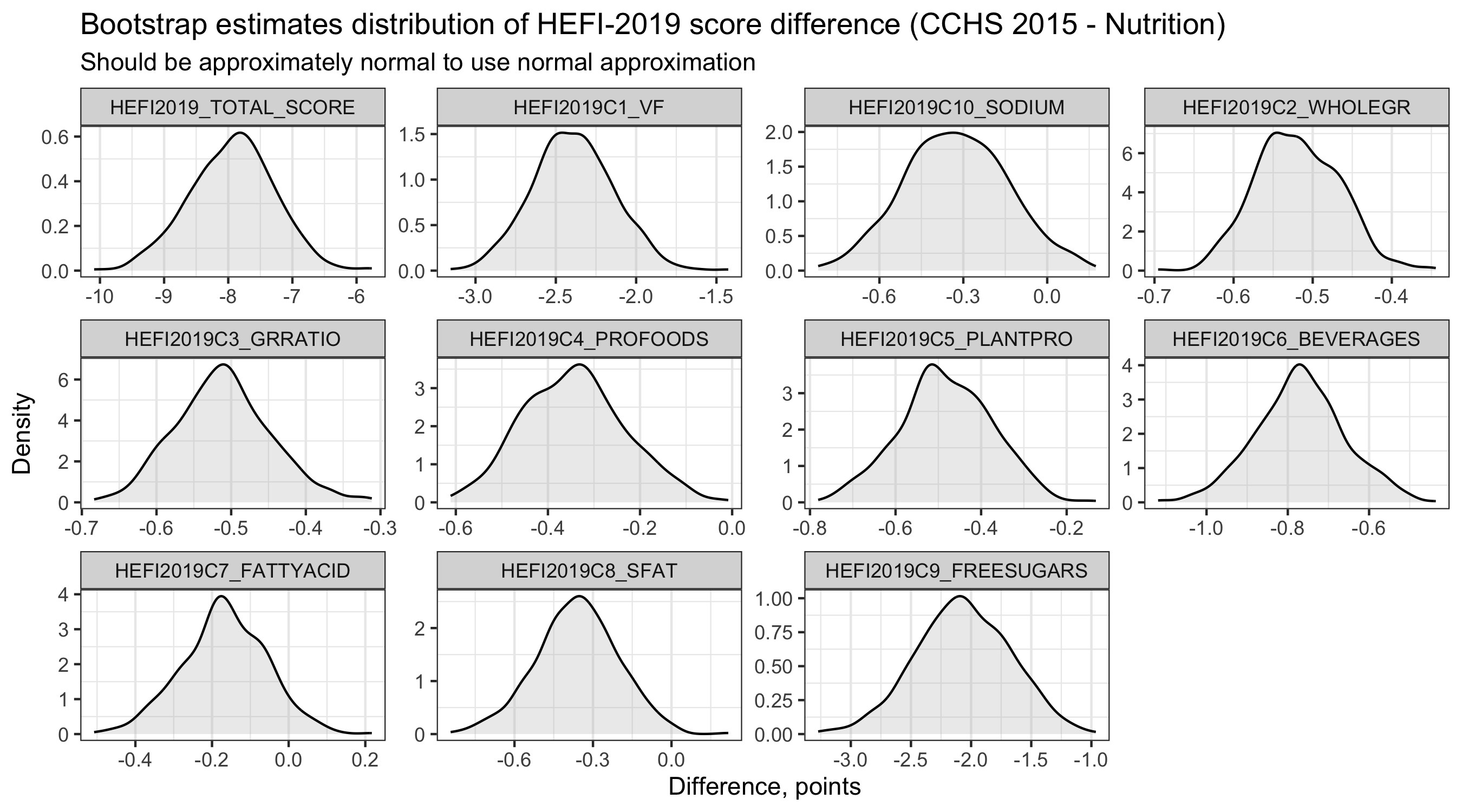
# 2) Check bootstrap estimates normality - best to look at when using normal approximation
hefi2019_smkbs |>
# note: I focus on difference for this example
ggplot(aes(x=DIFF)) +
geom_density(fill="gray",alpha=0.3) +
labs(title="Bootstrap estimates distribution for HEFI-2019 score difference (CCHS 2015 - Nutrition)",
subtitle = "Should be approximately normal to use normal approximation",
y="Density",x="Difference, points") +
facet_wrap(~HEFI2019_components,scales="free") +
theme_bw() +
theme( panel.grid.major.y = element_blank(),
legend.title = element_blank(),
legend.position = "top")
# 3) Calculate standard deviation of the sampling distribution (i.e., bootstrap Standard Error)

  hefi2019_smkbs_se <-
    hefi2019_smkbs |>
    group_by(HEFI2019_components) |>
    summarise(
      across(c("SMK_0","SMK_1","DIFF"), function(x) sd(x))
    )

# 4) Merge original sample estimates with bootstrap Standard Error, calculate 95CI

  # 4.1) Transpose base estimates (wide->long)
  hefi2019_smk0_long <-
    hefi2019_smk0 |>
    select(-replicate) |>
    pivot_longer(cols=c("SMK_0","SMK_1","DIFF"),
                 values_to="estimate")

  # 4.2) Transpose bootstraps Standard Error (wide->long)
  hefi2019_smkbs_se_long <-
    hefi2019_smkbs_se |>
    pivot_longer(cols=c("SMK_0","SMK_1","DIFF"),
                 values_to="se")

  # 4.3) Merge both data and calculate 95%CI using normal approximation
  hefi2019_smkf <-
    full_join(hefi2019_smk0_long, hefi2019_smkbs_se_long) |>
    mutate(
      # Calculate 95%CI
      nboot  = 500,
      alpha  = 0.05,
      tvalue = qt(1-(alpha/2),nboot-2),
      lcl    = estimate - (se * tvalue),
      ucl    = estimate + (se * tvalue)
    )

  # delete temporary data
  rm(list=c("hefi2019_smk0","hefi2019_smkbs",
            "hefi2019_smkbs_se","hefi2019_smk0_long",
            "hefi2019_smkbs_se_long"))

  # show final data
  head(hefi2019_smkf)
# A tibble: 6 × 9
  HEFI2019_components name  estimate     se nboot alpha tvalue    lcl    ucl
  <chr>               <chr>    <dbl>  <dbl> <dbl> <dbl>  <dbl>  <dbl>  <dbl>
1 HEFI2019C1_VF       SMK_0   10.1   0.126    500  0.05   1.96  9.86  10.4
2 HEFI2019C1_VF       SMK_1    7.85  0.224    500  0.05   1.96  7.41   8.29
3 HEFI2019C1_VF       DIFF    -2.25  0.253    500  0.05   1.96 -2.75  -1.76
4 HEFI2019C2_WHOLEGR  SMK_0    1.24  0.0341   500  0.05   1.96  1.18   1.31
5 HEFI2019C2_WHOLEGR  SMK_1    0.832 0.0434   500  0.05   1.96  0.746  0.917
6 HEFI2019C2_WHOLEGR  DIFF    -0.412 0.0529   500  0.05   1.96 -0.516 -0.309
We can then use the hefi2019smkf data frame to generate table or graph with results. I show a simple table below:
# ********************************************** #
#        Simple draft table with results         #
# ********************************************** #

  hefi2019_smkf |>
    mutate(
      # show estimate (95%CI) for difference and estimate (SE) for mean
      estimate_fmt =
        ifelse(name=="DIFF",
               paste0(round(estimate,1)," (", round(lcl,1),", ", round(ucl,1),")"),
               paste0(round(estimate,1)," (", round(se,2),")")
                )
    ) |>
    select(HEFI2019_components,name,estimate_fmt) |>
    # transpose data to wide format
    pivot_wider(values_from=estimate_fmt) |>
    # create table
    knitr::kable(
      col.names = c("HEFI-2019 components", "Non-smokers (SE)", "Smokers (SE)", "Difference (95%CI)"),
      caption = "Mean HEFI-2019 scores and difference in Smokers vs. Non-Smokers aged 19y+ (CCHS 2015 - Nutrition)")
| HEFI-2019 components | Non-smokers (SE) | Smokers (SE) | Difference (95%CI) |
|---|---|---|---|
| HEFI2019C1_VF | 10.1 (0.13) | 7.8 (0.22) | -2.3 (-2.8, -1.8) |
| HEFI2019C2_WHOLEGR | 1.2 (0.03) | 0.8 (0.04) | -0.4 (-0.5, -0.3) |
| HEFI2019C3_GRRATIO | 1.5 (0.04) | 1.1 (0.05) | -0.5 (-0.6, -0.3) |
| HEFI2019C4_PROFOODS | 5 (0.02) | 4.9 (0.11) | -0.1 (-0.3, 0.1) |
| HEFI2019C5_PLANTPRO | 1.8 (0.06) | 1.3 (0.09) | -0.4 (-0.7, -0.2) |
| HEFI2019C6_BEVERAGES | 7.9 (0.04) | 7.2 (0.1) | -0.7 (-1, -0.5) |
| HEFI2019C7_FATTYACID | 2.4 (0.05) | 2.2 (0.1) | -0.2 (-0.4, 0) |
| HEFI2019C8_SFAT | 4.2 (0.08) | 3.8 (0.14) | -0.4 (-0.7, -0.1) |
| HEFI2019C9_FREESUGARS | 9 (0.15) | 7.1 (0.38) | -1.9 (-2.6, -1.1) |
| HEFI2019C10_SODIUM | 5 (0.1) | 4.7 (0.16) | -0.3 (-0.7, 0.1) |
| HEFI2019_TOTAL_SCORE | 48.1 (0.34) | 40.9 (0.61) | -7.2 (-8.5, -5.9) |
Mean HEFI-2019 scores and difference in Smokers vs. Non-Smokers aged 19y+ (CCHS 2015 - Nutrition)
References
Brassard, D., Elvidge Munene, L. A., St-Pierre, S., Guenther, P. M., Kirkpatrick, S. I., Slater, J., Lemieux, S., Jessri, M., Haines, J., Prowse, R., Olstad, D. L., Garriguet, D., Vena, J., Vatanparast, H., L’Abbe, M. R., & Lamarche, B. (2022a). Development of the Healthy Eating Food Index (HEFI)-2019 measuring adherence to Canada’s Food Guide 2019 recommendations on healthy food choices. Appl Physiol Nutr Metab, 47(5), 595-610. https://doi.org/10.1139/apnm-2021-0415
Brassard, D., Elvidge Munene, L. A., St-Pierre, S., Gonzalez, A., Guenther, P. M., Jessri, M., Vena, J., Olstad, D. L., Vatanparast, H., Prowse, R., Lemieux, S., L’Abbe, M. R., Garriguet, D., Kirkpatrick, S. I., & Lamarche, B. (2022b). Evaluation of the Healthy Eating Food Index (HEFI)-2019 measuring adherence to Canada’s Food Guide 2019 recommendations on healthy food choices. Appl Physiol Nutr Metab, 47(5), 582-594. https://doi.org/10.1139/apnm-2021-0416
Freedman, L. S., Guenther, P. M., Krebs-Smith, S. M., & Kott, P. S. (2008). A population’s mean Healthy Eating Index-2005 scores are best estimated by the score of the population ratio when one 24-hour recall is available. J Nutr, 138(9), 1725-1729. https://doi.org/10.1093/jn/138.9.1725