
‘Statistical method you should know’: restricted cubic spline
Published:
In this article, I describe and provide a brief introduction for a statistical method that I find very useful: restricted cubic splines. During my PhD, I diligently learned regression models assumption for my biostatistics class. One of these assumptions in the case of linear regression models is that the independent variable \(X\) should be linearly related to the dependent variable, \(Y\). After all, it makes sense that linear regression models estimate linear relationships. I nearly fell off my chair when I learned that the linearity assumption is not even required! We can relax this assumption by using simple statistical transformations. One of those transformation is the restricted cubic spline.
Disclaimer: I have a PhD in nutrition, thus my knowledge of statistical methods is that of a naive enthusiast at best. I aim to provide a practical introduction based on my understanding. Please correct me where needed.

Of note, there are many options available to model a non-linear relationship (Bennette and Vickers, 2012), but restricted cubic splines offer some advantages which are discussed elsewhere (Desquilbet and Mariotti, 2010).
Why consider potential non-linearity?
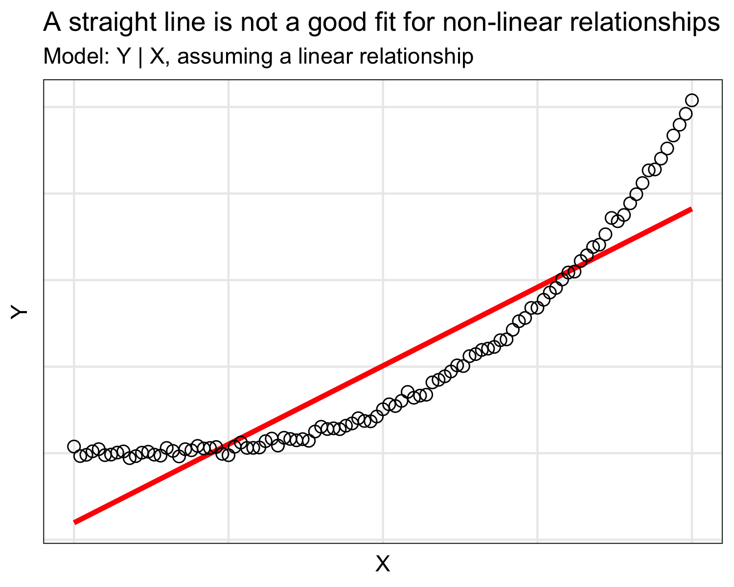
Typically for a linear regression model, we find the ‘best-fitted straight line’ through the data points. However, the ‘straight line’ (more commonly named ‘curve’) may not fit the data very well (Figure 1). Unsurprisingly, a straight curve does not adequately reflect non-linear relationships. The issue is that we often don’t know the shape of the ‘true’ relationship between the variables. This is what we are trying to estimate with the model after all! In sum, assuming linearity by default may obscure relationships and lead to erroneous conclusion (Khan et al. 2019).
What is a restricted cubic spline (RCS)?
Informally, a cubic spline is a transformation of a continuous independent variable which allows the curve to change shape smoothly at predetermined values. These predetermined values are called knots. Restricted means the curve is forced to be linear below and above the lower and upper knot, respectively. This is helpful to avoid overfitting the data.
For a more accurate definition and further details, see Prof. Harrell’s Regression Modeling Strategies book (Harrell, 2015).
How many knots and where?
A restricted cubic spline transformation is a flexible modelling strategy, yet, we don’t want to be too flexible. Having too many points at which the curve may change shape can cause overfitting of the data. In other words, we risk fitting a curve that is so specific to the data we have that it is no longer useful.
When applying a restricted cubic spline transformation, we have to decide the number of knots and their position. Unless background information is known about the importance of specific values, a popular heuristic scheme is to use 3 to 5 knots at predetermined quantiles (see table below from Harrell, 2015). Using quantiles that are well-distributed across the distribution ensures that there is enough information between knots to model the relationship. Sometimes, it may be useful to have more than 5 knots especially when dealing time or dates. However, in most cases, 3 to 5 knots will suffice.
| Number of knots | Position |
|---|---|
| 3 | .10 .50 .90 |
| 4 | .05 .35 .65 .95 |
| 5 | .05 .275 .50 .725 .95 |
| 6 | .05 .23 .41 .59 .77 .95 |
| 7 | .025 .1833 .3417 .5 .6583 .8167 .975 |
Additional terms
Once a restricted cubic spline transformation is applied to a single continuous variable, \(k-2\) additional variables are generated, where \(k\) = number of knots. These additional variables are then entered in the model together with the original variable. For example, the model equation:
\[Y_i=\beta_0+\beta_XX_i+\epsilon_i\]would become
\[Y_i=\beta_0+\beta_XX_i+\beta_X\prime X_i\prime +\beta_X\prime\prime X_i\prime\prime+\epsilon_i\]after a restricted cubic spline transformation with 4 knots is applied to \(X\). A total of 3 variables is used for \(X\), including 2 (\(k-2=2\)) additional ‘non-linear’ terms. In the second equation,
\(X_i\) is the original variable. \(\beta_X\) is the coefficient reflecting the linear relationship;
\(X_i\prime\) and \(X_i\prime\prime\) are derived from \(X\) for the transformation. \(\beta_X\prime\) and \(\beta_X\prime\prime\) are the coefficient reflecting the non-linear relationship, if any.
\(X_i\), \(X_i\prime\) and \(X_i\prime\prime\) are variables that together reflect the independent variable. \(\beta_X\), \(\beta_X\prime\) and \(\beta_X\prime\prime\) are regression coefficients reflecting the full relationship between \(X\) and \(Y\).
Notice that the model is slightly more complex after \(X\) has been transformed. In this example, modelling the independent variable with a restricted cubic spline requires 3 parameters instead of only 1. For smaller effective sample sizes, say \(n<100\), this is not a trivial issue, especially when there are multiple variables to be considered.
All in all, it is relevant to carefully decide a priori the number of knots while considering the effective sample size. With limited sample size, one potential strategy could be to allocate more knots to the main variable of interest, e.g.\(k=4\) or \(k=5\), but less to other variables that are less likely to have a major role, e.g., \(k=3\) or even assume linearity (no transformation).
Applying the transformation
While one could do the calculation by hand, statistical software offer simple solutions to apply the transformation including R (Perperoglou et al., 2019). Applying restricted cubic spline transformation using the built-in effect option in SAS is also possible for selected procedures.
Below, I demonstrate how we can apply restricted cubic spline transformation using the rms R package. For SAS users, I made a SAS tutorial about the use of restricted cubic spline.
Example use of restricted cubic spline in R
Data preparation and overview
To illustrate how restricted cubic spline may allow for flexible assessment of relationships, I use publicly available data from the Canadian Community Health Survey (CCHS) 2015 - Nutrition. I won’t go into much details about specifying the survey design to focus on restricted cubic splines transformation. I suggest reading my previous post if you need more details about the analysis of CCHS data. You can also skip to the next section
# ********************************************** #
#             Load required packages             #
# ********************************************** #

library(tidyverse)
library(data.table)
library(parallel)
library(survey)
library(haven)

# ********************************************** #
#         Load and prepare CCHS data: HS         #
# ********************************************** #

  # Note: a hardcoded path (<external_drive>) is used since files are on an external drive.
  # Usually we would want analysis to be self-contained, but survey files are a bit large.
  # Also, the data are set-up exactly as they are once obtained from Statistics Canada

# HS data file (includes energy intakes, age, sex, sampling weights)
cchs_data <-
  haven::read_sas(data_file = file.path(external_drive,"CCHS_Nutrition_2015_PUMF","Data_Donnee","hs.sas7bdat"),
                  col_select = c(ADM_RNO,WTS_P,DHH_AGE,DHH_SEX,PHSGAPA)) |>
  ## rename variables for simplicity
  dplyr::rename(AGE = DHH_AGE,
                SEX = DHH_SEX,
                PHYS_ACT_VIG = PHSGAPA) |>
  ## keep respondents aged 18-70y only, non-null energy
  dplyr::filter(AGE>=18, AGE<71) |>
  dplyr::mutate(
    ## create an indicator variable with value of 1 for sex=males, 0 otherwise
    MALE = ifelse(SEX==1,1,0),
    ## recode valid skip/not stated for physical activity data
    PHYS_ACT_VIG = ifelse(PHYS_ACT_VIG>20,NA,PHYS_ACT_VIG)
  )

# ********************************************** #
#         Load and prepare CCHS data: B5         #
# ********************************************** #

# Bootstrap replicate weights (for variance estimation)
 bsw <-
   data.table::fread(file.path(external_drive,"CCHS_Nutrition_2015_PUMF","Bootstrap",
                               "Data_Donnee","b5.txt"),
                     stringsAsFactors = F, data.table= F, header=F,
                     nThread = parallel::detectCores()-1, # note: a bit overkill, but why not
                     col.names = c("ADM_RNO","WTS_P",paste0("BSW",seq(1,500)))) |>
   # keep only respondents identified above
   dplyr::right_join(cchs_data[,"ADM_RNO"]) |>
   # remove sampling weights so that only 1 copy exists in <cchs_data>
   dplyr::select(-WTS_P)

 # ********************************************** #
#             Specify survey design              #
# ********************************************** #

  cchs_design_bsw <-
    survey::svrepdesign(
      data =  cchs_data, # HS data with variables of interest + sampling weights
      type = "bootstrap", # Replicate weights are bootstrap weights in CCHS
      weights    = ~WTS_P, # Sampling weights
      repweights = bsw[,2:501], # Bootstrap replicate weights (i.e. BSW1, BSW2, ... BSW500)
      combined.weights=TRUE,  # in CCHS 2015, weights are combined
      mse = TRUE # 'compute variances based on sum of squares around the point estimate' = same as in SAS
      )

# ********************************************** #
#              Check Survey Object               #
# ********************************************** #

cchs_design_bsw
Call: svrepdesign.default(data = cchs_data, type = "bootstrap", weights = ~WTS_P,
    repweights = bsw[, 2:501], combined.weights = TRUE, mse = TRUE)
Survey bootstrap with 500 replicates and MSE variances.
#Adapted from Statistics Canada, Canadian Community Health Survey - Nutrition: Public Use Microdata File, 2015, February 2023. This does not constitute an endorsement by Statistics Canada of this product.
Modelling and restricted cubic spline transformation
The data is a subset of respondents from the CCHS 2015 - Nutrition aged 18 to 70 years. In this analysis, I describe the relationship between age and sex (independent variables; AGE, MALE) and the reported number of hours per week of moderate/vigorous physical activity (dependent variable; PHYS_ACT_VIG). The linear regression model equation of the relationship is:
Once the restricted cubic spline transformation is applied to age (4 knots), the model equation becomes:
\[\text{PHYS_ACT_VIG}=\beta_0+\beta_{AGE}+\beta_{AGE}\prime+\beta_{AGE}\prime\prime+\beta_{MALE}+\epsilon\]Note that MALE is not transformed because it is a dummy variable (coded 0 or 1) and not a continuous variable like age. Also, to account for the survey design, I use the survey::svyglm function. For non-survey data, the base R glm function could be used by simply removing design = cchs_design_bsw.
# ********************************************** #
#             Load required packages             #
# ********************************************** #

library(rms) # rms library includes efficient function <rcs(x,k)> to recode variables
# parameters + marginaleffects library useful to visualize model output
library(parameters)
library(marginaleffects)

# ********************************************** #
#     Assess relationship with linear model      #
# ********************************************** #

svy_lm_rcs <-
  survey::svyglm(design = cchs_design_bsw,
                PHYS_ACT_VIG ~ rcs(AGE,4) + MALE,
                family = gaussian(link="identity") )

# print object
svy_lm_rcs
Call: svrepdesign.default(data = cchs_data, type = "bootstrap", weights = ~WTS_P,
    repweights = bsw[, 2:501], combined.weights = TRUE, mse = TRUE)
Survey bootstrap with 500 replicates and MSE variances.

Call:  survey::svyglm(design = cchs_design_bsw, formula = PHYS_ACT_VIG ~
    rcs(AGE, 4) + MALE, family = gaussian(link = "identity"))

Coefficients:
     (Intercept)    rcs(AGE, 4)AGE   rcs(AGE, 4)AGE'  rcs(AGE, 4)AGE''
         4.80080          -0.06851           0.16950          -0.51467
            MALE
         1.26006

Degrees of Freedom: 11436 Total (i.e. Null);  495 Residual
  (36 observations deleted due to missingness)
Null Deviance:      186800
Residual Deviance: 181600   AIC: 75240
# ********************************************** #
#           Generate model parameters            #
# ********************************************** #

svy_lm_rcs_parm <-
  parameters::model_parameters(svy_lm_rcs) |>
  as_tibble()

# print parameters
svy_lm_rcs_parm
# A tibble: 5 × 9
  Parameter Coefficient     SE    CI  CI_low CI_high Statistic df_error        p
  <chr>           <dbl>  <dbl> <dbl>   <dbl>   <dbl>     <dbl>    <dbl>    <dbl>
1 (Interce…      4.80   0.567   0.95  3.69    5.92        8.46      495 2.99e-16
2 rcs(AGE,…     -0.0685 0.0200  0.95 -0.108  -0.0291     -3.42      495 6.84e- 4
3 rcs(AGE,…      0.170  0.0563  0.95  0.0590  0.280       3.01      495 2.72e- 3
4 rcs(AGE,…     -0.515  0.179   0.95 -0.866  -0.163      -2.88      495 4.18e- 3
5 MALE           1.26   0.231   0.95  0.806   1.71        5.45      495 8.00e- 8
The intercept of the model \(\beta_0=\) 4.8 hours (95%CI, 3.7, 5.9) reflects the estimated number of hours of moderate and vigorous physical activity per week when AGE=0 and MALE=0, i.e., an average 19 y old female from Canada in 2015. The coefficient \(\beta_{MALE}=\) 1.3 hours (95%CI, 0.8, 1.7) is the additional number of hours males reported on average compared with females. But what do the coefficients \(\beta_{AGE}\), \(\beta_{AGE}\prime\) and \(\beta_{AGE}\prime\prime\) mean? Once a restricted cubic spline transformation is applied, we interpret the graph, not the coefficients!
Visualize model with a restricted cubic spline
The code below shows how to use the marginaleffects to generate predicted values from the model and how these values can be plotted with ggplot2.
# ********************************************** #
#     Generate predicted PHYS_ACT_VIG values     #
# ********************************************** #

curve <-
  marginaleffects::plot_predictions(model = svy_lm_rcs,
                                    condition =c("AGE","MALE"),
                                    draw=FALSE)

# ********************************************** #
#          Generate graph with ggplot2           #
# ********************************************** #

# apply formatting to male variables
curve$MALE_f <-
  factor(curve$MALE,
         levels =c(1,0),
         labels =c("Males","Females"))

# graph
ggplot(data=curve,aes(x=AGE,color=MALE_f)) +
  ## predicted values of the restricted cubic spline curve
  geom_line(aes(x=AGE,y=estimate),size=1.2) +
  ## 95% confidence intervals
  geom_line(aes(x=AGE,y=conf.low),linetype="longdash") +
  geom_line(aes(x=AGE,y=conf.high),linetype="longdash") +
  ## change default colors
  scale_color_manual("Sex",values=MetBrewer::met.brewer("Homer1",2)) +
  ## labels
  labs(x="Age, years",y="Moderate/vigorous physical activity, hours",
       title="Moderate/vigorous physical activity by age and sex in Canadians 18-70 y",
       subtitle="CCHS 2015 - Nutrition",
       caption = "Age modeled as a restricted cubic spline with 4 knots") +
  theme_bw() +
  theme(panel.grid.minor = element_blank())
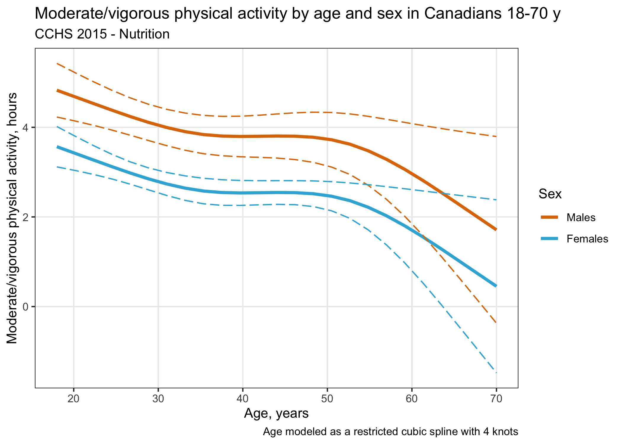
Based on Figure 2, we see the practice of moderate/vigorous physical activity is the highest between below 30 years of age, and decreases until approximately 35 y. There is a slight increase from the late 30s to approximately 50 y and then a sharp decrease until 70 y. Note that exact values can also be calculated.
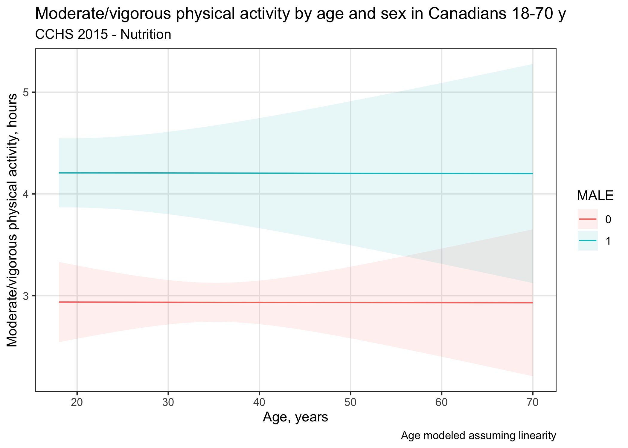
Finally, the graph produced by a linear regression model without the restricted cubic spline transformation would have shown a mostly null relationship. In other words, no evidence that age is related to reported moderate/vigorous physical activity (Figure 3)! Arguably, we would have missed important nuances had we assumed linearity without considering potential non-linearity.
# ********************************************** #
#     Assess relationship with linear model      #
# ********************************************** #

svy_lm_norcs <-
  survey::svyglm(design = cchs_design_bsw,
                PHYS_ACT_VIG ~ AGE + MALE,
                family = gaussian(link="identity") )


# ********************************************** #
#     Generate predicted PHYS_ACT_VIG values     #
# ********************************************** #

  marginaleffects::plot_predictions(model = svy_lm_norcs,
                                    condition =c("AGE","MALE"),
                                    draw=TRUE) +
  labs(x="Age, years",y="Moderate/vigorous physical activity, hours",
       title="Moderate/vigorous physical activity by age and sex in Canadians 18-70 y",
       subtitle="CCHS 2015 - Nutrition",
       caption = "Age modeled assuming linearity") +
  theme_bw() +
  theme(
     panel.grid.minor = element_blank()
  )
Reference
Bennette, C. & Vickers, A. (2012) Against quantiles: categorization of continuous variables in epidemiologic research, and its discontents. BMC Med Res Methodol, 12, 21. doi:10.1186/1471-2288-12-21.
Desquilbet, L. & Mariotti, F. (2010) Dose‐response analyses using restricted cubic spline functions in public health research. Statistics in Medicine, 29(9), 1037-1057. doi:10.1002/sim.3841.
Harrell, F. E. (2015) General Aspects of Fitting Regression Models, Regression Modeling Strategies: With Applications to Linear Models, Logistic and Ordinal Regression, and Survival Analysis. Cham: Springer International Publishing, 13-44.
Khan, T. A., Chiavaroli, L., Zurbau, A. & Sievenpiper, J. L. (2019) A lack of consideration of a dose-response relationship can lead to erroneous conclusions regarding 100% fruit juice and the risk of cardiometabolic disease. Eur J Clin Nutr, 73(12), 1556-1560. doi:10.1038/s41430-019-0514-x.
Perperoglou, A., Sauerbrei, W., Abrahamowicz, M. & Schmid, M. (2019) A review of spline function procedures in R. BMC Med Res Methodol, 19(1), 46. doi:10.1186/s12874-019-0666-3.