
‘Statistical method you should know’: percentage difference
Published:
For descriptive purpose, we may want to plot and compare many differences for variables with varying units. Nutrient intakes are a common example where we may have data measured in calories (e.g., energy), grams (e.g., saturated fats) or servings (e.g., sugar-sweetened beverages). However, the extent of the difference - the effect size - cannot be easily compared when units and scales vary. Percentage difference and log-transformation of data may be helpful to facilitate result presentation.
In addition, data transformation are commonly used to better satisfy assumptions of regression models. The log transformation is helpful, given that it is interpreted correctly.
Types of percentage difference
Traditional
Typically, the percentage difference is calculated as a difference over a reference value. For example, say we measured mean energy intake intake in a control group (group=0; 2500 kcal) as well as in an intervention group (group=1; 3000 kcal), we may calculate the percentage difference in mean energy as:
\[\text{percentage}_\text{diff.}=\frac{X_1-X_0}{X_0}\cdot100\]For the example above, \(X\) is the energy intake and the (traditional) percentage difference is
\[\frac{3000-2500}{2500}=\frac{500}{2500}\cdot100=20\%\]However, the choice of the reference value is not always straightforward, especially when there is no clear time ordering or reference value. For example, had we decided to use the mean energy intake of group 1 as the reference, we would have obtained a 16.7% percentage difference.
Reference invariant
An alternative percentage difference that does not vary according to the choice of the reference value is (Cole & Altman, 2017a):
\[\text{percentage}_\text{diff.}=\frac{X_1-X_0}{\mu_{(X_0, X_1)}}\cdot100\]where \(\mu\) is the mean. For the example above, the (symmetrical) percentage difference is
\[\frac{3000-2500}{\mu_{(3000,2500)}}=\frac{500}{2750}=18.2\%\]This alternative calculation does not depend on which value we use as reference and is symmetrical.
Unfortunately, both the traditional and reference invariant difference have an important drawback: they are not additive.
Log-based
Cole & Altman (2017b) present an elegant solution based on log-transformation: “if we take two numbers a and b, then the difference between their logs, \(ln(a)−ln(b)\), is the fractional difference between a and b”.
For all values greater than zero, we can use this convenient natural logarithm rule to calculate percentage difference. Of note, the use of natural logarithm for this task is important as it will circumvent the need to back-transform the difference. In other words, using natural logarithm permits a direct interpretation of the result (Cole, 2000).
\[\text{percentage}_\text{diff.}=({ln(X_1)-ln(X_0)}) \cdot 100\]For the example above, the (symmetrical and additive) log-based percentage difference is
\[({\text{ln}(3000)-\text{ln}(2500)})\cdot100=(8.01-7.82)\cdot100=19\%\]This alternative calculation does not depend on the reference value. It is also symmetrical and additive. More details are available regarding this property of the natural logarithm (Cole, 2000).
Example application: difference of means between two groups
Nutrient intake data are good candidates for the log transformation as nutrient intake values are always positive and most often greater than zero. For example, nutrient intake differences between two groups can be calculated on a common percentage scale by 1) calculating log values of the nutrients for the two groups, and 2) then the difference of the log-transformed nutrient values between groups. The percentage differences can then be plotted on a common axis, which helps us appreciate the extent of differences.
Another feature of data transformation is to better satisfy linear regression model assumptions. For example, one may transform a continuous \(Y\) to \(\text{log}(Y)\) to obtain model errors that are approximately identically and normally distributed. Contrary to other transformations, the log transformation is the only transformation that can have an intuitive interpretation once we back-transform (i.e, take the antilog or exponentiate) the effect estimates obtained based on log-transformed outcome data. Furthermore, using natural logarithm (\(\text{log}_e(Y)\) or \(\text{ln}(Y)\)) also circumvent the need to back-transform data as described above (Cole, 2000).
Simulation
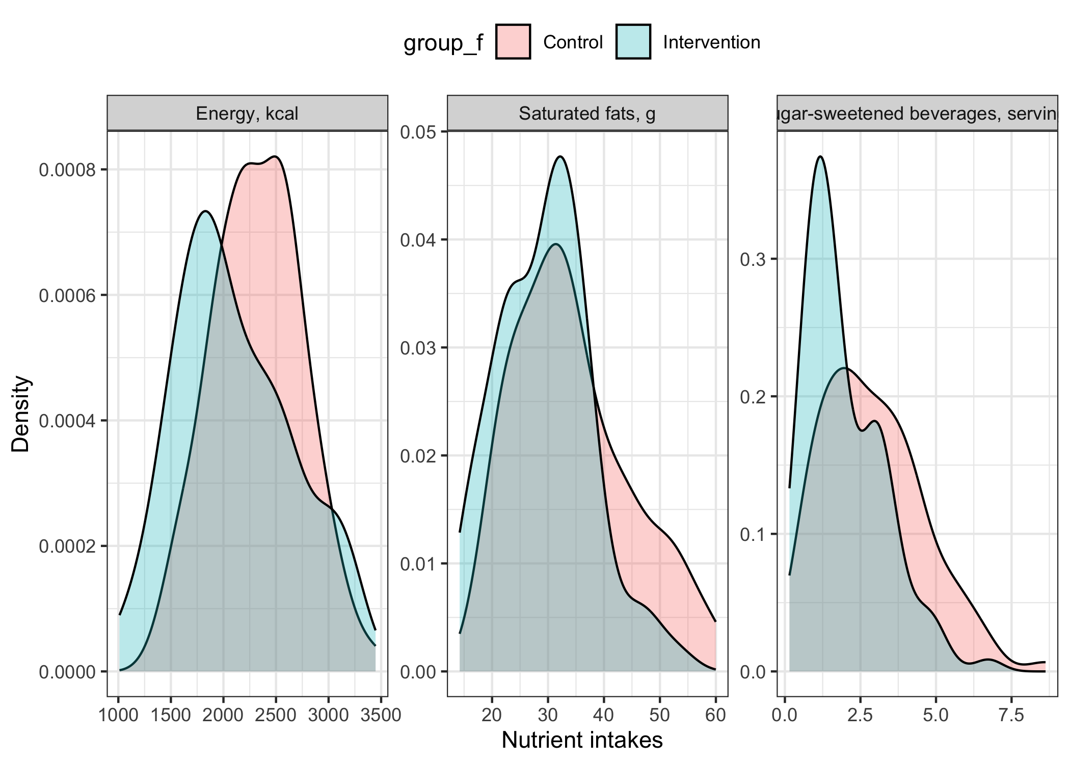
For demonstration purpose, I simulate nutrient intake data with varying units: energy in calories, saturated fats in grams and sugar-sweetened beverages in servings. In this example, there are two groups, i.e., a control and intervention group. For both groups, we have estimated nutrient intakes and we wish to know the difference in nutrient intakes between groups.
On the original scale, plotting all differences would not be informative. On the log-transformed scale, the percentage difference makes it easy to compare effect size estimates. All in all, the log transformation may improve model robustness and facilitate result presentation.
Figure 1 presents an overview of the distribution among the two groups.
# load package
library(dplyr)
library(parameters)
library(ggplot2)
library(gtsummary)

# ********************************************** #
#              Simulation function               #
# ********************************************** #

# function to simulate gamma data with given mean and standard deviation
custom_gamma <- function(sample_size, mean_value, sd_value){
# generate right-skewed data using rgamma function with mean and sd values
right_skewed_data <-
  rgamma(n = sample_size,
         shape = (mean_value/sd_value)^2,
         scale = sd_value^2/mean_value)
return(right_skewed_data)
}

# ********************************************** #
#           Simulate and prepare data            #
# ********************************************** #

# Simulation of three variables for two groups

## Group 0, i.e., simulated controls
set.seed(1)
group_0 <-
  data.frame(
    group   = 0,
    energy  = custom_gamma(100,2300,500), # kcal
    sfa     = custom_gamma(100,35,10),    # grams
    ssbs    = custom_gamma(100,2.9,1.8)   # servings
      )

## Group 1, i.e., simulated intervention
set.seed(2)
group_1 <-
  data.frame(
    group   = 1,
    energy  = custom_gamma(100,2100,500), # kcal
    sfa     = custom_gamma(100,30,8),     # grams
    ssbs    = custom_gamma(100,1.7,1.2)   # servings
      )

## append both data together
sim_intervention <-
  rbind(group_0, group_1)

# add group label - useful for a nicer output with <gtsummary>, <ggplot2>
sim_intervention$group_f <-
  factor(sim_intervention$group,
         levels = c(0,1),
         labels = c("Control","Intervention"))

# add variable labels - useful for a nicer output with <gtsummary>
labelled::var_label(sim_intervention) <-
  list(group   = "Group identifier",
       group_f = "Group identifier",
       energy  = "Total energy, kcal/d",
       sfa     = "Saturated fats, g/d",
       ssbs    = "Sugar-sweetened beverages, serving/d")

# ********************************************** #
#         Summary of data using ggplot2          #
# ********************************************** #

# make labels for <facet_wrap>
facet_labels <-
  c(energy = "Energy, kcal",
   sfa = "Saturated fats, g",
   ssbs ="Sugar-sweetened beverages, servings")

# Check raw data distribution
sim_intervention |>
  ## transform to long-formatted data for ggplot
  tidyr::pivot_longer(
    cols = c(energy, sfa, ssbs)
  ) |>
ggplot(aes(x=value,fill=group_f)) +
  geom_density(alpha = 0.3)  +
  facet_wrap(~name,scales="free",labeller=as_labeller(facet_labels)) +
  labs(x="Nutrient intakes", y="Density") +
  theme_bw() +
  theme(legend.position = "top")
The table presents mean intakes as well as difference on the original scale.
# ********************************************** #
#        Difference on the original scale        #
# ********************************************** #

sim_intervention |>
  select(-group) |>
gtsummary::tbl_summary(
  by = group_f,
  statistic =
    all_continuous() ~ c( "{mean} ({sd})" )
  ) |>
  gtsummary::add_difference() |>
  gtsummary::as_kable()
| Characteristic | Control, N = 100 | Intervention, N = 100 | Difference | 95% CI | p-value |
|---|---|---|---|---|---|
| Total energy, kcal/d | 2,323 (423) | 2,108 (548) | 215 | 78, 351 | 0.002 |
| Saturated fats, g/d | 34 (10) | 29 (8) | 5.0 | 2.4, 7.6 | <0.001 |
| Sugar-sweetened beverages, serving/d | 2.92 (1.67) | 1.96 (1.29) | 0.96 | 0.55, 1.4 | <0.001 |
Mean food and nutrient intakes and difference between groups
At this point, we have successfully calculated differences among groups (assuming no confounding, no selection bias and no measurement error). Although a table could suffice, I like graph.
Percentage difference using linear regression models
In the code below, I use a linear regression model to estimate the difference in nutrient intakes between groups. The linear regression model has the equation:
\[\text{log}_e\text{(nutrient)}_i=\beta_0+\beta_\text{Group}\text{Group}_i+\epsilon_i\]Since nutrients are expressed on the log scale, a change of 1 unit for any independent variable now reflect a change in \(\text{log}_e\text{(nutrient)}\), i.e., a percent difference! Indeed, \(\text{log}(a) - \text{log}(b) = \text{log} (\frac{a}{b})\)
# package to loop analysis
library(purrr)

# ********************************************** #
#           Function for linear model            #
# ********************************************** #

  # note: use a function to have consistent output

output_diff <- function(outcome,log=FALSE){
  # outcome : nutrient for which we want to know differences
  # log     : TRUE/FALSE indicating if outcome should be log-transformed

if(log==FALSE){
  # no transformation = raw data as outcome
model <- lm(sim_intervention[,outcome]~group, data=sim_intervention)
}else {
  # transformation = log outcome data (natural log by default)
model <- lm(log(sim_intervention[,outcome])~group,
            data=sim_intervention)
}
# the <parameters> function extract reg. coef. + 95CI
# function can also back-transform (i.e., exponentiate) data
return(
  tibble::as_tibble(parameters::parameters(model,exponentiate=FALSE)) |>
    dplyr::mutate(outcome = ) |>
    dplyr::filter(Parameter=="group") |>
    dplyr::select(outcome, Parameter, Coefficient, CI_low, CI_high)
)
}

# ********************************************** #
#             Calculate differences              #
# ********************************************** #

# list outcome values
my_nutrients <- c("energy", "sfa", "ssbs")

# loop <my_nutrients through the <output_diff> function
lm_diff_log <-
  purrr::map(.x  = my_nutrients,
           .f  = output_diff,
           log = TRUE) |>
  ## append the output data of each call
  purrr::list_rbind()

# show data
lm_diff_log
# A tibble: 3 × 5
  outcome Parameter Coefficient CI_low CI_high
  <chr>   <chr>           <dbl>  <dbl>   <dbl>
1 energy  group          -0.114 -0.178 -0.0500
2 sfa     group          -0.155 -0.237 -0.0722
3 ssbs    group          -0.443 -0.643 -0.242
Back-transformation
On one hand, natural logarithms were used in the example above to avoid the need for a back-transformation. Natural logarithms are calculated by default in R. On the other hand, had we used a different base for the log transformation, say log10, the regression coefficient should have been back-transformed to be interpreted as a percent difference.
Linear regression coefficients for a change in \(\text{log}_{10}\) outcome can be back-transformed using the following equation:
\[\text{Percentage}_\text{diff.}=100 \cdot 10^{\beta_{X}}-100\]where \(\beta_{X}\) represents the estimated regression coefficient based on log-transformed outcome.
The same equation can also be used for the \(\text{log}_\text{e}\) transformation:
\[\text{Percentage}_\text{diff.}=100 \cdot e^{\beta_{X}}-100\]For example, we can back-transform the regression coefficient for the simulated energy variable (\(\beta_X=\) -0.114) using the R code 100*exp(lm_diff_log[1,3])-100. We find that the estimated percent difference in total energy intake between group is -11%. This result is similar to the untransformed regression coefficient, since the natural logarithm was used.
Results and interpretation
Once percentage differences are calculated based on log-transformed data, it is finally possible to plot and compare effect estimate on a common axis.
# ********************************************** #
#               Plot using ggplot2               #
# ********************************************** #

# make nicer label
lm_diff_log$outcome_f <-
  factor(lm_diff_log$outcome,
         levels = lm_diff_log$outcome,
         labels = c("Total energy",
         "Saturated fats",
         "Sugars-sweetened beverages"))

# combine estimate with 95%CI
lm_diff_log |>
  mutate(
    estimate_ci = paste0(
      scales::percent(Coefficient,accuracy=0.1),
      " (",scales::percent(CI_low,accuracy=0.1),", ",
      scales::percent(CI_high,accuracy=0.1),")")
  )  |>
  # plot data and text
  ggplot(aes(x=outcome_f,y=Coefficient)) +
  geom_point() + # point estimate
  geom_linerange(aes(ymin=CI_low,ymax=CI_high)) + # 95%CI
  geom_hline(yintercept=0,linetype="longdash", color="gray")+ #null value
  geom_text(aes(label=estimate_ci), size=3, nudge_x = 0.1) +
  scale_y_continuous(labels = scales::percent_format(accuracy = 0.1)) +
  labs(x=NULL, y="Symmetric percentage difference") +
  coord_flip() +  # switch axis for clarity
  theme_bw(base_size=14)
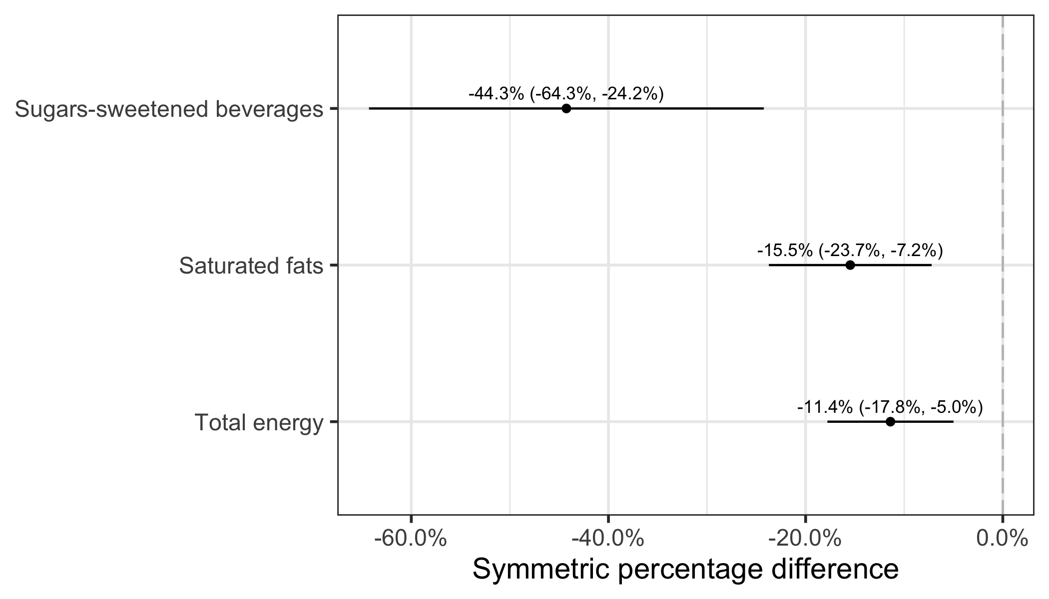
In conclusion, Figure 2 clearly shows that the mean difference is much larger for sugar-sweetened beverages than for energy intake, followed by saturated fats. These observations were not explicit based on values on the original scale.
As a final note, I want to point out that instead of a regression model, I could have either calculated the “crude” difference between groups (difference of mean of log data) and/or used a t test (t.test(log(energy) ~ group, data= sim_intervention)). The results would have been exactly the same as the linear regression model. The linear model has the advantage of being more flexible, since covariates can easily be added, although not shown in my example.
References
Cole, T. J., & Altman, D. G. (2017a). Statistics Notes: What is a percentage difference? BMJ, 358, j3663. https://doi.org/10.1136/bmj.j3663
Cole, T. J., & Altman, D. G. (2017b). Statistics Notes: Percentage differences, symmetry, and natural logarithms. BMJ, 358, j3683. https://doi.org/10.1136/bmj.j3683
Cole, T. J. (2000). Sympercents: symmetric percentage differences on the 100 log(e) scale simplify the presentation of log transformed data. Stat Med, 19(22), 3109-3125. https://doi.org/10.1002/1097-0258(20001130)19:22<3109::aid-sim558>3.0.co;2-f