
The most boring yet essential skill (part 2): reshaping data
Published:
A common data manipulation task involves transposing data from a long (portrait) to wide (landscape) format, and vice versa. This manipulation is sometimes necessary to accommodate statistical procedure, but also to aggregate and combine variables in a data. In nutrition, a typical example is combining repeated dietary intake data. For example, study participant may have completed 2 or 3 24-hour dietary recalls each and we may wish to calculate average intakes among repeated assessments. While this manipulation can be done manually in Excel, having reproducible code is advantageous for many reasons. The purpose of this blog is to introduce these common data format and demonstrate how we can go from one format to another using R, as well as nutrition data example.
The distinction between long and wide data only becomes relevant with repeated data. That is, when there is more than one data collection among study participants. When we collect multiple dietary assessment (e.g., 24-hour dietary recalls, food recods, or food-frequency questionnaire), we will have repeated observations for each participant. When we collect data at different timepoints (e..g, baseline, 3 months, 6 months, …), we will also have repeted observations for each participant. On the contrary, if we only have a single assessment at a single point in time for each participant, and that those participants are not related or grouped, both long and wide data are equivalent because there is no repeated information.
The difference between long vs. wide data format
Long (portrait) data
In a long data, repeated information are stored vertically as shown in Table 1.
| Participant_id | Assessment | Food_1 | Food_2 | Food_3 | Food_j… |
|---|---|---|---|---|---|
| 1 | First | 2 | 1 | 9 | … |
| 1 | Second | 1 | 3 | 4 | … |
| 2 | First | 4 | 4 | 5 | … |
| 2 | Second | 2 | 1 | 3 | … |
| 3 | First | 2 | 7 | 6 | … |
| 3 | Second | 4 | 3 | 6 | … |
| 4 | First | 5 | 4 | 5 | … |
| 4 | Second | 5 | 2 | 7 | … |
| 5 | First | 6 | 4 | 2 | … |
| 5 | Second | 4 | 3 | 5 | … |
Table 1: Data in the long format where repeated assessments appear vertically
The long format simplifies variable names especially when there are many, since the index of the repeated assessment appears as a variable on its own. This is an advantage of this format that may facilitate data manipulation. The number of repeated assessment per individual is easy to obtain, often directly with basic procedure.
# How many assessment per participant?
table(data_long$Assessment)
 First Second
     5      5
I find relatively easier to transform data from the long format to the wide format (next). In doubt, I suggest you opt for a long format to collect or prepare your data.
Wide (landscape) data
In a wide data, repeated information are stored horizontally as shown in Table 2. Notice that only one observation per Participant_id appears on each row despite having two assessments. The wide format requires including the index of the repeated assessment in each variable’s name, which makes variable naming slightly more cumbersome.
| Participant_id | Food_1_First | Food_1_Second | Food_2_First | Food_2_Second | Food_3_First | Food_3_Second | Food_j…_First | Food_j…_Second |
|---|---|---|---|---|---|---|---|---|
| 1 | 2 | 1 | 1 | 3 | 9 | 4 | … | … |
| 2 | 4 | 2 | 4 | 1 | 5 | 3 | … | … |
| 3 | 2 | 4 | 7 | 3 | 6 | 6 | … | … |
| 4 | 5 | 5 | 4 | 2 | 5 | 7 | … | … |
| 5 | 6 | 4 | 4 | 3 | 2 | 5 | … | … |
Table 2: Data in the wide format where repeated assessments appear horizontally
The advantage of the wide data is that operations across repeated assessment are relatively easier to perform, e.g., mean of Food_1_First and Food_1_Second. The wide format also simplifies merging manipulation, especially when we wish to combine data that do not include repeated assessment (e.g., participant characteristics that would not change like baseline age or biological sex) with data that include repeated assessment (e.g., the repeated dietary data as shown above).
The number of (unique) individuals is easy to obtain in the wide format. Using nrow(data_wide), we find that there are 5 individuals.
With such a small data, the benefits of learning code are not obvious. However, reshaping data from hundreds of participants, each with multiple repeated assessment and many variables, would be very hard to perform efficiently and without errors. The next section illustrates how code can be used to reshape such data.
Simulated data for demonstration
In this example, I use a simulated data named dietary_data which includes 1000 participants, each with 3 repeated measurements, and 3 dietary variables named energy, fiber, and vf. To show a data similar to that of real life, 5% of participants have missing values for recalls on day 2 or day 3. All in all, the data look similar to summary intakes one would get after collecting repeated food records or 24-hour dietary recalls for example. Of note, the data currently appears in the long format, where repeated observations are stored vertically.
Table 3 presents means, standard deviation, min and max values of variables in dietary_data.
# General overview
dim(dietary_data); names(dietary_data); head(dietary_data); table(dietary_data$day)
[1] 3000    5

[1] "participant" "day"         "energy"      "fiber"       "vf"

# A tibble: 6 × 5
# Rowwise:
  participant   day energy fiber    vf
        <int> <dbl>  <dbl> <dbl> <dbl>
1           1     1  1828.  14.4  2.79
2           2     1  2750.  15.2  5.60
3           3     1  3153.  40.0  5.38
4           4     1  2067.  27.4  7.17
5           5     1  1820.  23.2  8.30
6           6     1  2468.  17.1  5.13


   1    2    3
1000 1000 1000
# Summary intakes using the gtsummary package
library(gtsummary)

dietary_data[-1] |>
  gtsummary::tbl_summary(
    by = day, # day = the index of dietary recall
    type = all_continuous() ~ "continuous2",
    statistic = list(all_continuous() ~ c("{mean} ({sd})", "[{min}, {max}]") )
  ) |>
  gtsummary::as_kable()
| Characteristic | 1, N = 1,000 | 2, N = 1,000 | 3, N = 1,000 |
|---|---|---|---|
| Energy intake, kcal/day | |||
| Mean (SD) | 2,308 (430) | 2,290 (419) | 2,287 (418) |
| [Range] | [968, 3,733] | [858, 3,837] | [1,188, 3,633] |
| Unknown | 0 | 50 | 50 |
| fiber | |||
| Mean (SD) | 20 (7) | 20 (7) | 20 (7) |
| [Range] | [0, 49] | [0, 45] | [1, 40] |
| Unknown | 0 | 50 | 50 |
| vf | |||
| Mean (SD) | 5.17 (1.70) | 5.08 (1.68) | 5.05 (1.70) |
| [Range] | [0.00, 11.11] | [0.00, 9.83] | [0.35, 11.71] |
| Unknown | 0 | 50 | 50 |
Table 3: Descriptive statistics of the simulated dietary_data data
Reshape from long to wide
Suppose we wish to calculate mean intake values based on the 3 dietary recalls, but we also want to retain the information of each recall individually. Before calculating mean inakes, we would have to transpose data.
I find the pivot_wider function from tidyr package is the simplest solution for this task. New variable names have to include the repeated observation identifier, i.e. the recall index in this example (variable=day). The new variable names will have the following general structure: X_r1, X_r2, X_r3 for recalls 1, 2, and 3, respectively, and where X is replaced by energy, fiber, or vf.
# ********************************************** #
#           Reshape from wide to long            #
# ********************************************** #

library(tidyr)

dietary_data_w <-
  dietary_data |>
  tidyr::pivot_wider(
    values_from = c("energy", "fiber", "vf"), # i.e., the columns we wish to transpose
    names_from  = "day", # i.e., the index for the repeated observations (here, dietary recall)
    names_sep   = "_",   # i.e., the separator between <values_from> and <names_prefix>
    names_prefix = "r"   # i.e., any characters added before the value from <names_from> and after <names_sep>
  )

# overview
dim(dietary_data_w); names(dietary_data_w); head(dietary_data_w)
[1] 1000   10

 [1] "participant" "energy_r1"   "energy_r2"   "energy_r3"   "fiber_r1"
 [6] "fiber_r2"    "fiber_r3"    "vf_r1"       "vf_r2"       "vf_r3"

# A tibble: 6 × 10
  participant energy_r1 energy_r2 energy_r3 fiber_r1 fiber_r2 fiber_r3 vf_r1
        <int>     <dbl>     <dbl>     <dbl>    <dbl>    <dbl>    <dbl> <dbl>
1           1     1828.     1809.     2162.     14.4     14.3     18.9  2.79
2           2     2750.     2607.     2532.     15.2     22.2     10.2  5.60
3           3     3153.     2754.     2944.     40.0     36.0     39.3  5.38
4           4     2067.     2060.     2585.     27.4     36.5     28.5  7.17
5           5     1820.     1902.     2334.     23.2     18.4     27.0  8.30
6           6     2468.     2437.     2635.     17.1     21.7     23.7  5.13
# ℹ 2 more variables: vf_r2 <dbl>, vf_r3 <dbl>
As you can see, reshaping data from long to wide can be done with only a few lines of code. For this reason, I prefer to have my “analysis-ready” data in this format rather than in the wide format. We can now summarize intakes based on recall-specific variables.
There are many different methods (base R, tidyverse) to calculate row-wise means, i.e., the mean values between the columns in the data for each observation or participant.
Calculate row-wise means with base R
First, here is one base R approach using rowMeans. Note that na.rm=TRUE must be added, otherwise, participants with missing day 2 or day 3 would all have NA for mean energy.
# ********************************************** #
#      Calculate mean energy inake - base R      #
# ********************************************** #

# Calculate mean energy intakes using base R
energy_mean_r123 <-
  rowMeans(dietary_data_w[c("energy_r1", "energy_r2", "energy_r3")], na.rm=TRUE)

# Summary
summary(energy_mean_r123)
   Min. 1st Qu.  Median    Mean 3rd Qu.    Max.
   1166    2050    2278    2293    2515    3665
Calculate row-wise means with tidyverse
Second, here is the tidyverse approach which I use more often because I find it easier to scale up for many variables or many recalls.
# ********************************************** #
#    Calculate mean energy inake - tidyverse     #
# ********************************************** #

# load library for mutate, and others
library(dplyr)

# Calculate mean energy intakes using tidyverse approach
dietary_data_w_mean <-
  dietary_data_w |>
  dplyr::rowwise() |> # note: indicates that the averaging process should be performed across observations rather than columns
  dplyr::mutate(
     "energy_mean_r123" := mean(dplyr::c_across(dplyr::starts_with("energy")),na.rm=TRUE)
  )

  # warning: there shouldn't be variables with a name that start with 'energy' beyond the recall-specific values.

# Summary
summary(dietary_data_w_mean$energy_mean_r123)
   Min. 1st Qu.  Median    Mean 3rd Qu.    Max.
   1166    2050    2278    2293    2515    3665
Both base R and tidyverse approach give the same values in the end.
Using a function
Ideally, we would push this one step further and create a function to easily calculate or means for different variables. The advantages of using a function are 1) you can re-use the function for future analyses; 2) you can more easily add new variables without copy/pasting; 3) you only have to change code once if you need to expanded the function (i.e., calculate other statistics than average) or if you made an error at some point. Here is a brief example of such function and its application to calculate mean intakes.
# ********************************************** #
#         1) Function to calculate means         #
# ********************************************** #

library(dplyr)

calculate_mean <- function(data, variable_prefix){
data_with_mean <-
  data |>
  dplyr::rowwise() |> # note: indicates that the averaging process should be performed across observations rather than columns
  dplyr::mutate(
    "{paste0(variable_prefix,'_mean')}" := mean(dplyr::c_across(dplyr::starts_with(variable_prefix)),na.rm=TRUE)
  ) |>
  dplyr::select(ends_with('_mean'))

return(data_with_mean)

}

# ********************************************** #
#      2) Create vector of variable prefix       #
# ********************************************** #

variable_prefixes <- c("energy", "fiber", "vf")

# ********************************************** #
#      3) use <lapply> to loop the function      #
# ********************************************** #

result_list <-
  lapply(variable_prefixes, function(prefix) {
    calculate_mean(data = dietary_data_w, variable_prefix = prefix)
  })

# ********************************************** #
#            4) prepare a final data             #
# ********************************************** #

means_among_recalls <-
  dplyr::bind_cols(result_list)

# Merge with data including recall-specific values
dietary_data_w_means <-
 cbind(dietary_data_w,means_among_recalls)

# Overview
dim(dietary_data_w_means); names(dietary_data_w_means)
[1] 1000   13

 [1] "participant" "energy_r1"   "energy_r2"   "energy_r3"   "fiber_r1"
 [6] "fiber_r2"    "fiber_r3"    "vf_r1"       "vf_r2"       "vf_r3"
[11] "energy_mean" "fiber_mean"  "vf_mean"
Final summary of the average values
Table 4 presents means, standard deviation, min and max values of variables in dietary_data_w_means.
dietary_data_w_means[,c("energy_mean", "fiber_mean", "vf_mean")] |>
  gtsummary::tbl_summary(
    type = all_continuous() ~ "continuous2",
    statistic = list(all_continuous() ~ c("{mean} ({sd})", "[{min}, {max}]") )
  ) |>
  gtsummary::as_kable()
| Characteristic | N = 1,000 |
|---|---|
| energy_mean | |
| Mean (SD) | 2,293 (348) |
| [Range] | [1,166, 3,665] |
| fiber_mean | |
| Mean (SD) | 20.0 (5.9) |
| [Range] | [4.9, 44.3] |
| vf_mean | |
| Mean (SD) | 5.11 (1.41) |
| [Range] | [0.99, 10.06] |
Table 4: Descriptive statistics of the average intakes among recalls in dietary_data data
Reshape from wide to long
It is not uncommon to have data stored in the wide format. In this case, we may wish to transpose variables so they appear in the long format which is often required for statistical procedure or visualization purpose. For this process, the key is having consistent variable names.
Say we have one variable for energy intake measured over 3 dietary recalls:
- Consistent naming pattern:
energy_r1,energy_r2,energy_r3 - Inconsistent naming pattern:
day1_energy,Day2_Energy,energyDaythree
Hopefully, this is already the case and you don’t have to change many variable names. However, if you face inconsistent naming pattern, the package janitor and janitor::clean_names() might be useful to save time.
Another consideration is to keep only the variables you want to transpose and necessary identifiers. In the present example, this means participant (participant identifier) and the dietary variables of interest with recall index. If you have multiple time points each with multiple recalls, you would have to keep the time point identifier variable to track which records belong at which time point (not shown here).
# overview of the wide data - making sure names are consistent
dim(dietary_data_w); names(dietary_data_w); head(dietary_data_w,10)
[1] 1000   10

 [1] "participant" "energy_r1"   "energy_r2"   "energy_r3"   "fiber_r1"
 [6] "fiber_r2"    "fiber_r3"    "vf_r1"       "vf_r2"       "vf_r3"

# A tibble: 10 × 10
   participant energy_r1 energy_r2 energy_r3 fiber_r1 fiber_r2 fiber_r3 vf_r1
         <int>     <dbl>     <dbl>     <dbl>    <dbl>    <dbl>    <dbl> <dbl>
 1           1     1828.     1809.     2162.     14.4     14.3     18.9  2.79
 2           2     2750.     2607.     2532.     15.2     22.2     10.2  5.60
 3           3     3153.     2754.     2944.     40.0     36.0     39.3  5.38
 4           4     2067.     2060.     2585.     27.4     36.5     28.5  7.17
 5           5     1820.     1902.     2334.     23.2     18.4     27.0  8.30
 6           6     2468.     2437.     2635.     17.1     21.7     23.7  5.13
 7           7     2719.     2532.     2122.     19.0     21.1     12.8  6.04
 8           8     2384.     2791.       NA      30.4     25.3     NA    5.68
 9           9     2785.     1824.     2759.     29.2     22.9     27.8  8.44
10          10     2006.     2428.     2581.     20.6     32.8     31.4  4.12
# ℹ 2 more variables: vf_r2 <dbl>, vf_r3 <dbl>
I find the pivot_longer function from tidyr package is the simplest solution as it works in the opposite direction than pivot_wider.
# ********************************************** #
#           Reshape from wide to long            #
# ********************************************** #

library(tidyr)

dietary_data_l <-
  dietary_data_w |>
  pivot_longer(
    cols = names(dietary_data_w)[-1], # i.e., the variable we want to transpose = all, but <participant> (first)
    names_to  = "variable", # i.e., the name of the column where original variable names are copied
    values_to = "value" # i.e., the name of the column where variable values are copied
  )

# overview
dim(dietary_data_l); names(dietary_data_l); head(dietary_data_l,10)
[1] 9000    3

[1] "participant" "variable"    "value"

# A tibble: 10 × 3
   participant variable    value
         <int> <chr>       <dbl>
 1           1 energy_r1 1828.
 2           1 energy_r2 1809.
 3           1 energy_r3 2162.
 4           1 fiber_r1    14.4
 5           1 fiber_r2    14.3
 6           1 fiber_r3    18.9
 7           1 vf_r1        2.79
 8           1 vf_r2        3.57
 9           1 vf_r3        4.15
10           2 energy_r1 2750.
We see the format of the dietary_data_l data is even “longer” than the original long data we had. We could say that we have reshaped from a wide format to a long-long format. In some cases, the long-long may be exactly what you need. For demonstration purpose, I show how to go back to the original (simple) long data.
# ********************************************** #
#         Reshape from long-long to long         #
# ********************************************** #

# load package
library(dplyr)
library(tidyr)

# Go back to original version of <dietary_data>
dietary_data_original <-
  dietary_data_l |>
  # 1) split variable names and recall index
  tidyr::separate_wider_delim(
    cols = variable,
    delim = "_",
    names = c("varname", "recall_index")
    ) |>
  # 3) reshape from long-long to (simple) long
  pivot_wider(
    names_from = "varname", # i.e., the column that has the variable names
    values_from = "value"   # i.e., the column that has the variable values
  )

# overview
dim(dietary_data_original); names(dietary_data_original); head(dietary_data_original, 10)
[1] 3000    5

[1] "participant"  "recall_index" "energy"       "fiber"        "vf"

# A tibble: 10 × 5
   participant recall_index energy fiber    vf
         <int> <chr>         <dbl> <dbl> <dbl>
 1           1 r1            1828.  14.4  2.79
 2           1 r2            1809.  14.3  3.57
 3           1 r3            2162.  18.9  4.15
 4           2 r1            2750.  15.2  5.60
 5           2 r2            2607.  22.2  5.08
 6           2 r3            2532.  10.2  3.70
 7           3 r1            3153.  40.0  5.38
 8           3 r2            2754.  36.0  5.50
 9           3 r3            2944.  39.3  6.55
10           4 r1            2067.  27.4  7.17
Conclusion
I hope these examples help you save some time if you need to perform these common manipulations. Sometimes, I find it difficult to intuitively know the results of a given reshaping procedure beforehand. Thus, I may use trial and errors until I can obtain the desired format. To avoid the headache of obtaining a given format, I recommend investing time into creating functions that do exactly what you need, so that you can re-use these procedures in your project.
The flow chart below summarizes the tidyverse-way of reshaping dietary intake data.
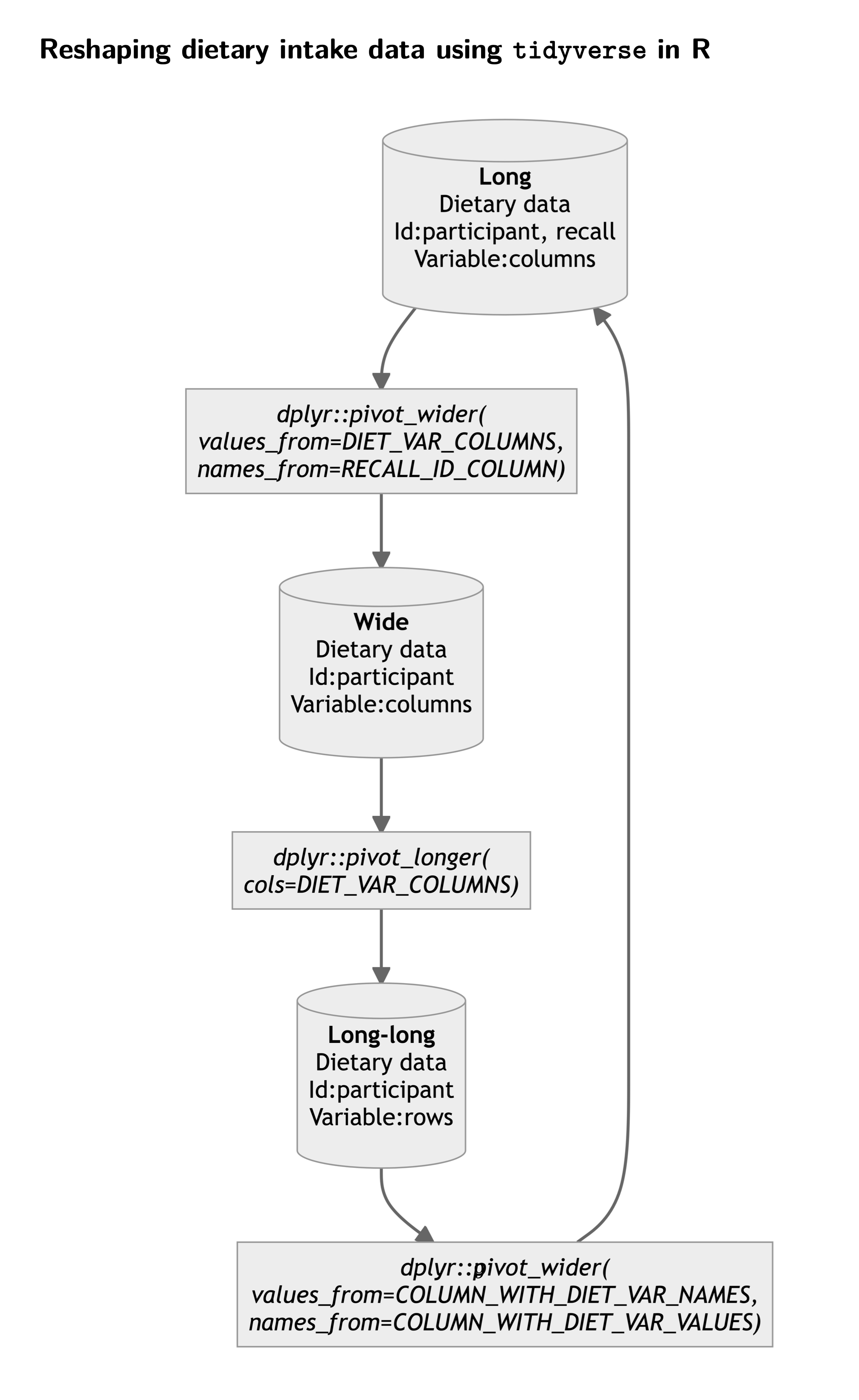
Finally, if you need to perform these manipulations on very large dataset, it may be worth using the data.table package and the data.table::dcast function in particular for a significant gain in processing speed.